We are excited to share the materials for our data engineering and exploratory data analysis (EDA) session: Advanced Data Manipulation & EDA with Pandas: Preprocessing for Machine Learning.
This session serves as the critical bridge from raw data to scikit-learn models, showing you how to shape and clean feature matrices ($X$) and target vectors ($y$).
🚀 Presentation Resources
Session Outline & Pre-ML Preprocessing Blueprint
Below is the complete lesson blueprint and scheduling outline for the session.
Target Audience: Data Professionals transitioning to Machine Learning & Scikit-Learn
Format: 1-Hour Live Session (Interactive Code Walkthrough + Conceptual Slides)
Speakers: Aakash Khandelwal & Tarun Garg
Deliverable: A single, comprehensive master guide detailing block timelines, slide structures, presenter scripts, visual aids, coding patterns, and ML-preparation checkpoints.
💡 Pre-ML Focus: The Bridge to Scikit-Learn
To prepare the audience for the upcoming classical Machine Learning classes (Supervised Regression/Classification, Unsupervised Clustering, and Model Evaluation), this session highlights:
- Handling Missing Values (
NaN): Traditional Scikit-Learn estimators cannot ingest missing data. We teach detection and Pandas imputation strategies (.fillna(),.dropna()). - Categorical Encoding: Converting string columns to numeric representation (
pd.get_dummies()and.map()) so Scikit-Learn models can process them. - Feature-Target Splitting: Using Pandas indexers to split datasets into $X$ (feature matrix) and $y$ (target vector).
- GroupBy Aggregations: Engineering features by grouping transactional data (
Split-Apply-Combine) and calculating rolling statistics. - Time Series Feature Extraction: Constructing numerical features (day of week, lag, lead, rolling averages) from raw dates, enabling models to predict future trends.
- EDA for Model Selection: Checking target distributions (
value_counts()) and feature correlations (.corr()) to identify multicollinearity before training linear models.
⏱️ 60-Minute Block Schedule
| Time | Slide Range | Block Name | Focus | ML Prep Relevance |
|---|---|---|---|---|
| 00:00 – 00:08 | Slides 1 – 4 | 01. Kickoff: Pandas in the ML Pipeline | DataFrames, Series, Ecosystem Alternates | Understanding data shapes ($X$ and $y$) and multi-core engines. |
| 00:08 – 00:20 | Slides 5 – 8 | 02. Data Cleaning & ML Data Prep | NaNs, duplicates, data types, categorical mapping | Preventing Scikit-Learn execution crashes. |
| 00:20 – 00:30 | Slides 9 – 11 | 03. Filtering & Transformations | Filtering, .apply(), Lambdas, NumPy np.where | Custom feature engineering and scaling. |
| 00:30 – 00:33 | Slide 12 | 04. Interactive Concept Quiz 1 | Spot-the-Prep-Bug | Rapid quiz to debug code block issues before ML. |
| 00:33 – 00:43 | Slides 13 – 15 | 05. Combining Data & GroupBy Aggregations | Merge, Join, Concat, GroupBy aggregates | Joining feature tables & creating group-level features. |
| 00:43 – 00:53 | Slides 16 – 18 | 06. Time Series & Dates for ML | Datetime index, lag/lead (.shift()), rolling | Building lagged target features for forecasting. |
| 00:53 – 00:58 | Slides 19 – 21 | 07. EDA & Visualization with Seaborn | Target imbalance, correlations, outlier boxplots | Identifying multicollinearity & classification class imbalances. |
| 00:58 – 01:00 | Slide 22 | 08. Recap & Scikit-Learn Handover | Preprocessing checklist & Pandas 3.0 roadmap | Cheatsheet: mapping Pandas code to Scikit-Learn tasks. |
01. Kickoff: Pandas in the ML Pipeline (00:00 – 00:08)
Slide 1: Welcome & Roadmap
Slide Title: Advanced Pandas & Seaborn: The Preprocessing Engine for Machine Learning

Welcome Cover Image
Slide 2: Pandas Internals vs. Polars & DuckDB
- Slide Title: The Data Ecosystem: Pandas, Polars & DuckDB
- Core Concepts:
- Pandas Constraints: Single-core/single-threaded execution (leaves modern CPU power idle) and in-memory execution (requires 5-10x dataset size in RAM, causing memory crashes on big data).
- Polars: Rust-backed, multi-threaded CPU parallelization, lazy query plan optimization, and streaming execution for larger-than-RAM tables.
- DuckDB: In-process serverless columnar SQL engine, optimized for aggregations and direct querying of Parquet/CSV files without full RAM loads.
Slide 3: DataFrame vs. Series Anatomy
Slide Title: Anatomy of Pandas Data Structures
Core Concepts:
- Series (1D): A single labeled array. Maps to the target vector ($y$) in Scikit-Learn.
- DataFrame (2D): A tabular structure with aligned row and column indexes. Maps to the feature matrix ($X$) in Scikit-Learn.
- Indexes: Row labels (
df.index) vs. column headers (df.columns). The critical role of alignment in operations.
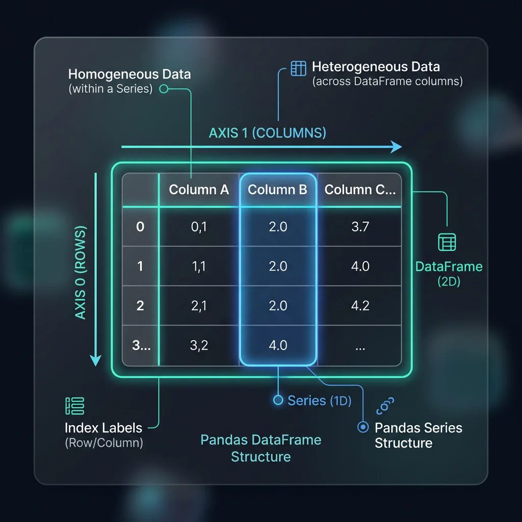
DataFrame vs Series Anatomy
Slide 4: The Data Pipeline Blueprint
Slide Title: The Data Preparation Pipeline for Scikit-Learn
Core Concepts:
- Visualizing the workflow: Raw Data $\rightarrow$ Pandas Cleaning $\rightarrow$ Seaborn EDA $\rightarrow$ Scikit-Learn Pipeline.
- Why Scikit-Learn requires homogeneous, non-null, numerical matrices.
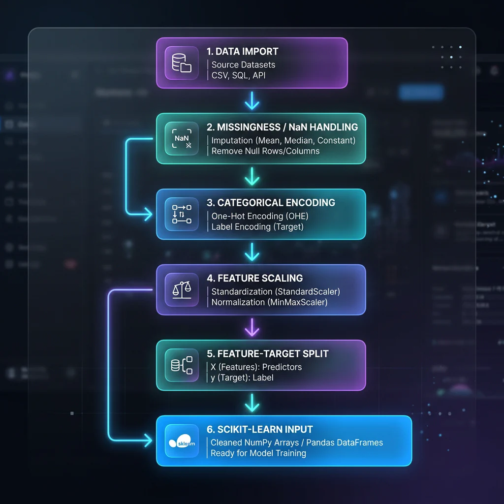
Data Preprocessing Pipeline Flowchart
02. Data Cleaning & ML Data Prep (00:08 – 00:20)
Slide 5: The NaN Problem in Machine Learning
Slide Title: Handling Missing Values (NaN)
Core Concepts:
- Why does Scikit-Learn throw
ValueError: Input contains NaN? - Detection:
df.isnull().sum()to find missing values. - Action 1: Dropping:
df.dropna(subset=['target'])- when to delete rows or columns. - Action 2: Imputation:
df.fillna(value)- replacing NaNs with median/mean/mode to preserve sample size.
- Why does Scikit-Learn throw
Python Implementation:
# Check missing values in customer profiles
print(df_customers.isnull().sum())

# Impute missing Customer Age with the column median
median_age = df_customers['age'].median()
df_customers['age'] = df_customers['age'].fillna(median_age)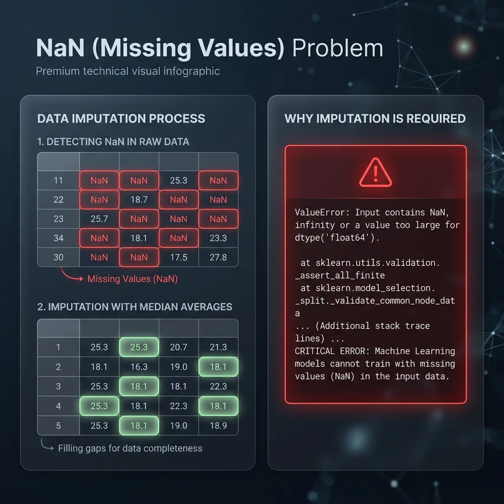
Handling Missing Values (NaN)
Slide 6: Duplicate and Format Resolution
- Slide Title: Data Integrity: Duplicates & Casts
- Core Concepts:
- Duplicate rows leak information between training/testing splits, inflating accuracy metrics (data leakage).
- Detecting duplicates:
df.duplicated().sum(). - Removing duplicates:
df.drop_duplicates(keep='first'). - Data type inspection:
.dtypesand casting with.astype(). Converting object strings to categories/floats.
- Python Implementation:
# Check duplicate count
dup_count = df_transactions.duplicated().sum()

# De-duplicate rows
df_transactions = df_transactions.drop_duplicates(keep='first')

# Cast columns for memory and math efficiency (Category types)
df_mem_opt = df_customers.copy()
df_mem_opt['membership'] = df_mem_opt['membership'].astype('category')
df_mem_opt['gender'] = df_mem_opt['gender'].astype('category')
Slide 7: Categorical Encoding (One-Hot Encoding)
Slide Title: Encoding Categorical Data
Core Concepts:
- ML models require numbers, not strings. How to convert text groups.
- One-Hot Encoding: Creating binary dummy variables for nominal data.
- Ordinal Mapping: Mapping ranked categories (e.g., ‘Bronze’, ‘Silver’, ‘Gold’) to integers (
[0, 1, 2]) using.map(). - Avoiding the Dummy Variable Trap: dropping the first category (
drop_first=True) to prevent multicollinearity.
Python Implementation:
# Ordinal mapping
membership_map = {'Bronze': 0, 'Silver': 1, 'Gold': 2}
df_customers['membership_encoded'] = df_customers['membership'].map(membership_map)

# Nominal encoding (One-Hot Encoding)
df_customers_encoded = pd.get_dummies(df_customers, columns=['gender'], drop_first=True)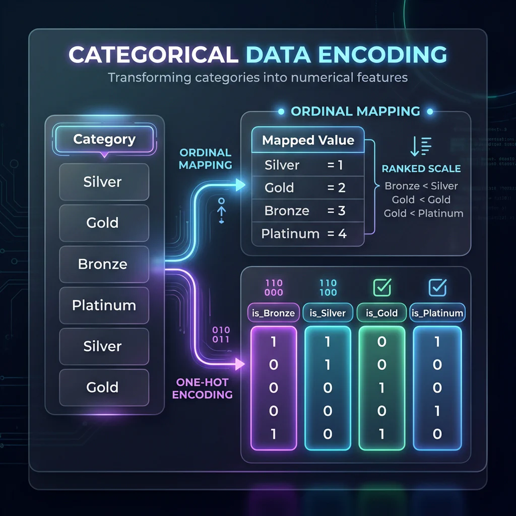
Categorical Data Encoding
Slide 8: Feature-Target Splitting ($X$ and $y$)
- Slide Title: Splitting Features ($X$) and Target ($y$)
- Core Concepts:
- Splitting columns into inputs ($X$ DataFrame) and labels ($y$ Series) before passing to Scikit-Learn.
- Using column drops vs. indexers (
.loc,.iloc).
- Python Implementation:
# Drop ID labels and string/date objects that are not encoded
features_to_drop = [
    'transaction_id', 'customer_id', 'category',
    'membership', 'signup_date', 'is_fraud',
    'target_lead_1h', 'spend_group'
]

# Split into Feature Matrix X and Target vector y
X = df_ts.drop(columns=features_to_drop)
y = df_ts['is_fraud']
03. Filtering & Transformations (00:20 – 00:30)
Slide 9: Boolean Indexing & Advanced Filtering
- Slide Title: Filtering DataFrames
- Core Concepts:
- Selecting specific observations for model subgroups (e.g., isolating high-value customers).
- Syntax rules: Boolean conditions, element-wise operators (
&,|,~), and.query()for clean, readable code.
- Python Implementation:
# Filter using bitwise operators
high_value_electronics = df_transactions[
    (df_transactions['category'] == 'Electronics') & (df_transactions['amount'] > 150)
]

# Filter using query syntax (equivalent)
high_value_electronics = df_transactions.query("category == 'Electronics' and amount > 150")
Slide 10: Custom Feature Engineering: Lambda Functions
- Slide Title: Row-wise Operations with
.apply()andlambda - Core Concepts:
- Creating new features using custom functions on columns.
- The syntax of
lambda x: expression. - Performance warning:
.apply(axis=1)is slow for large datasets because it loops over rows.
- Python Implementation:
# Create a custom premium fee feature based on category
df_transactions['premium_fee'] = df_transactions.apply(
    lambda row: row['amount'] * 0.05 if row['category'] == 'Electronics' else row['amount'] * 0.02,
    axis=1
)
Slide 11: Vectorized Transformations with NumPy
- Slide Title: Vectorization: Fast Transformations with NumPy
- Core Concepts:
- Why vectorization is $100\times$ faster than Lambda/Apply.
- NumPy helper functions:
np.where()for binary conditions, andnp.select()for multi-condition cases. - Creating target classes (e.g., binning continuous scores into binary flags for classification).
- Python Implementation:
import numpy as np

# Fast Vectorized Categorization using np.where()
df_transactions['is_high_value'] = np.where(df_transactions['amount'] > 150, 1, 0)

# Multi-class Categorization using np.select()
conditions = [
    df_transactions['amount'] < 80,
    (df_transactions['amount'] >= 80) & (df_transactions['amount'] < 150),
    df_transactions['amount'] >= 150
]
choices = ['Low_Spend', 'Medium_Spend', 'High_Spend']
df_transactions['spend_group'] = np.select(conditions, choices, default='Unknown')
04. Interactive Concept Quiz 1 (00:30 – 00:33)
Slide 12: Spot-the-Prep-Bug Quiz
- Slide Title: Interactive Quiz: Debug the ML Preprocessing Code
- Core Concepts:
- Reviewing a snippet of code containing errors that would crash Scikit-Learn or corrupt model training.
- Audit Items:
- Running One-Hot encoding but forgetting to drop target labels or categorical strings.
- Failing to handle NaNs before fitting.
- Splitting $X$/$y$ incorrectly.
05. Combining Data & GroupBy Aggregations (00:33 – 00:43)
Slide 13: Concatenation vs. Merging vs. Joining
Slide Title: Combining Datasets: The Core Joins
Core Concepts:
- Concatenation (
pd.concat): Stacking datasets vertically (adding rows/samples) or horizontally (adding columns/features). - Merging (
pd.merge): SQL-style key-based joins (matching columns). - Joining (
df.join): Index-based merges (matching row indices).

Merge and Join Concept Image - Concatenation (
Slide 14: SQL-Style Merging in Action
- Slide Title: Database-Style Merges
- Core Concepts:
- Matching tables (e.g.
df_transactionsjoined withdf_customersoncustomer_id). - Determining the join type:
how='left': Retains all transactions, filling customer profiles with NaN if missing (vital for preserving transaction history).how='inner': Drops transactions without matching customer profiles.
- Matching tables (e.g.
- Python Implementation:
# SQL-style Left Join to attach customer features to transaction records
df_merged = pd.merge(df_transactions, df_customers_encoded, on='customer_id', how='left')
Slide 15: GroupBy & Aggregations (Split-Apply-Combine)
Slide Title: Aggregating & Grouping Data
Core Concepts:
- Split: Segmenting the DataFrame based on a categorical key column.
- Apply: Computing aggregations (like mean, sum, or count) using
.agg(). - Combine: Merging the results back into a summarized DataFrame.
- Advanced: Group Centering (
.transform()): Calculating group-level stats and broadcast-mapping them to individual rows to engineer relative features.
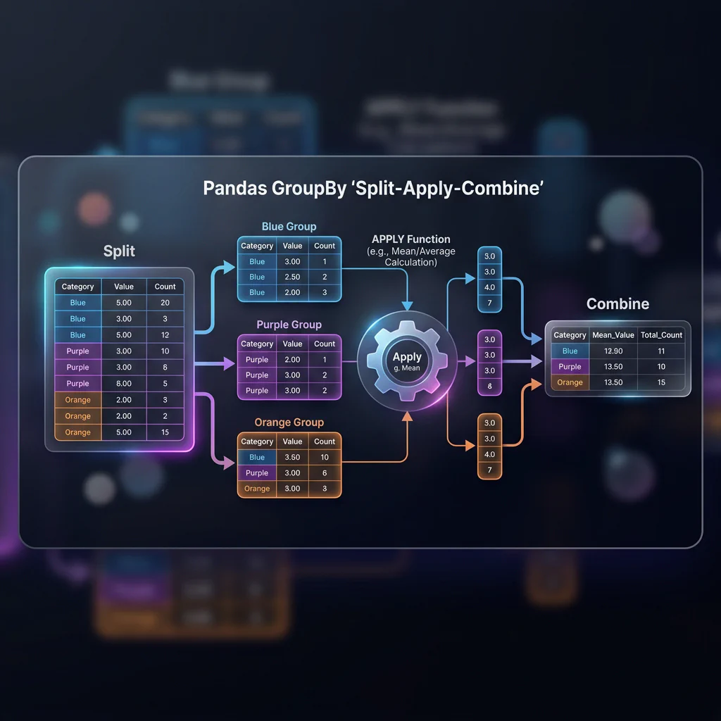
GroupBy Split-Apply-Combine Python Implementation:
# Basic grouping and mean calculation
group_means = df_merged.groupby('membership')['amount'].mean()

# Multi-column aggregation using .agg()
agg_results = df_merged.groupby('membership').agg({
    'amount': ['mean', 'max', 'std'],
    'age': 'median'
})

# Group centering for feature engineering
df_merged['amount_diff_tier_mean'] = df_merged['amount'] - df_merged.groupby('membership')['amount'].transform('mean')
06. Time Series & Dates for ML (00:43 – 00:53)
Slide 16: Datetime Conversions & Feature Extraction
Slide Title: Engineering Numerical Features from Dates
Core Concepts:
- ML models cannot ingest timestamps. We must extract numerical patterns.
- Parsing strings to date-time objects:
pd.to_datetime(). - Extracting date parts:
dt.year,dt.month,dt.day,dt.dayofweek,dt.hour. - Boolean indicators:
dt.dayofweek // 5 == 1(identifying weekends).
Python Implementation:
# Parse dates and extract numerical features
df_merged['timestamp'] = pd.to_datetime(df_merged['timestamp'])
df_merged['hour'] = df_merged['timestamp'].dt.hour
df_merged['day_of_week'] = df_merged['timestamp'].dt.dayofweek
df_merged['is_weekend'] = np.where(df_merged['day_of_week'] >= 5, 1, 0)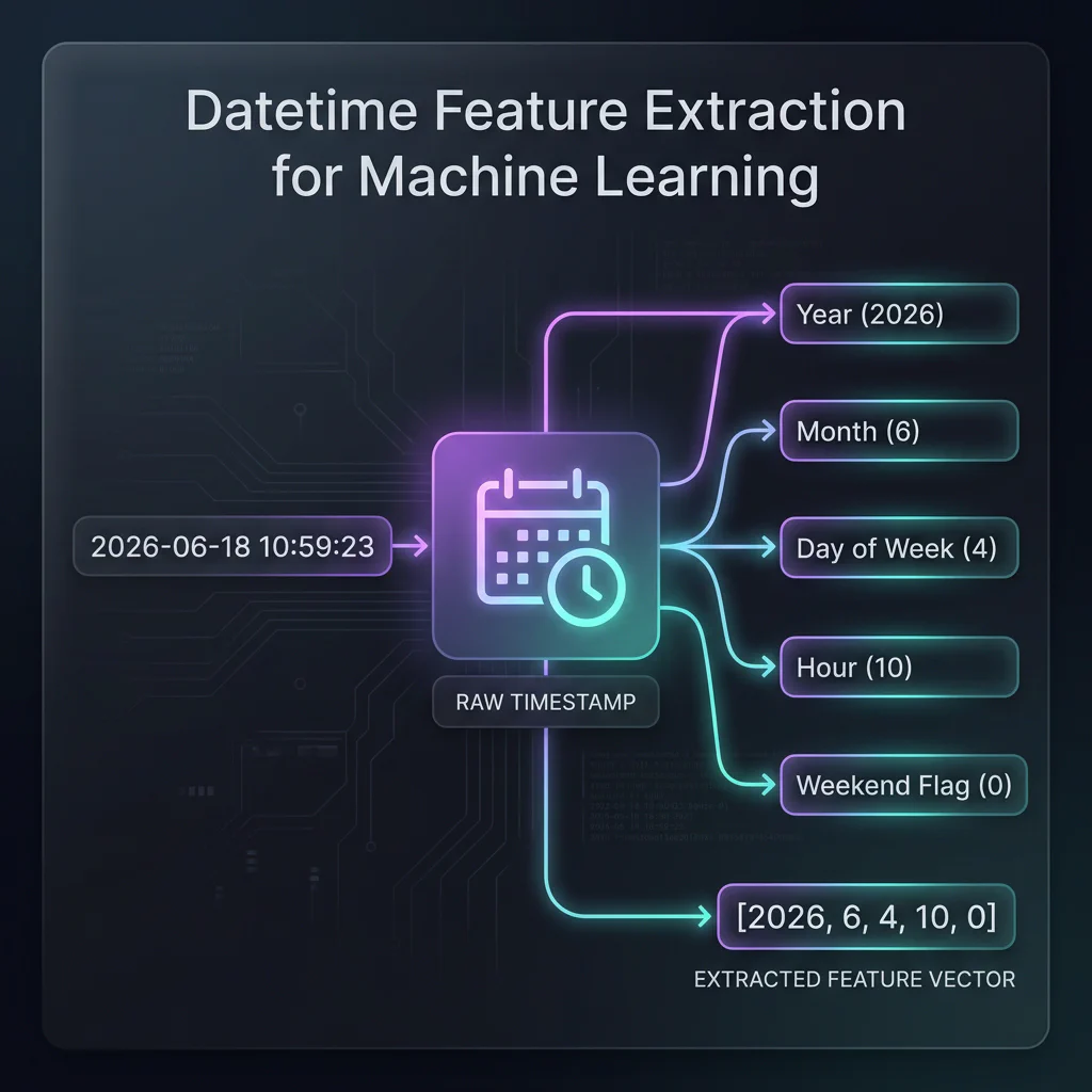
Datetime Feature Extraction
Slide 17: Time Series Indexing & Shifting (Lag/Lead)
Slide Title: Auto-Regressive Features: Lag & Lead
Core Concepts:
- Time series forecasting models learn patterns from past values.
- Lag (
.shift(1)): Moving values forward in time (using yesterday’s price to predict today’s). - Lead (
.shift(-1)): Moving values backward in time. Useful for constructing supervised labels (predicting tomorrow’s price).
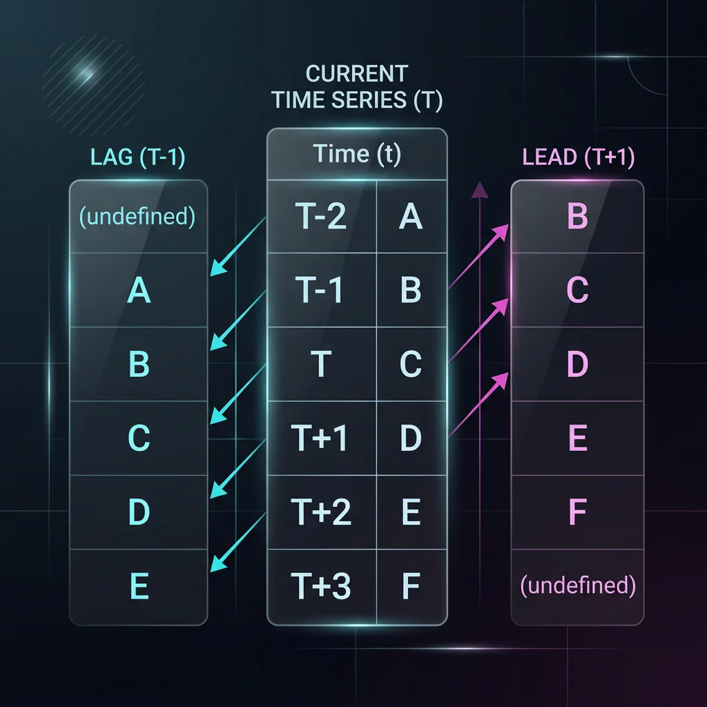
Lag and Lead Timeline Image Python Implementation:
# Set index to datetime and sort for timeline alignment
df_ts = df_merged.set_index('timestamp').sort_index()

# Lag features (past value predictors)
df_ts['lag_amount_1h'] = df_ts['amount'].shift(1)
df_ts['lag_amount_2h'] = df_ts['amount'].shift(2)

# Lead target (tomorrow's value to predict)
df_ts['target_lead_1h'] = df_ts['amount'].shift(-1)
Slide 18: Rolling Window Aggregations
- Slide Title: Rolling Window Features
- Core Concepts:
- Smoothing noisy time series signals.
- Generating rolling features:
df.rolling(window). - Compiling moving averages or moving standard deviations.
- Python Implementation:
# 3-period rolling average
df_ts['rolling_mean_3h'] = df_ts['amount'].rolling(window=3).mean()

# 14-day rolling standard deviation (volatility)
df_ts['rolling_std_14d'] = df_ts['amount'].rolling(window='14d').std()
07. EDA & Visualization with Seaborn (00:53 – 00:58)
Slide 19: Summary Statistics & Target Imbalances
Slide Title: Exploratory Data Analysis (EDA) basics & Target Imbalance
Core Concepts:
- Describing feature scales and bounds using
df.describe(). - Checking target balance for classification:
df['label'].value_counts(normalize=True). - The Accuracy Paradox: In highly imbalanced datasets, a model can achieve very high accuracy by simply predicting the majority class.
- Why Pandas audits inform ML metrics: identifying class imbalance during EDA warns the data scientist not to use simple accuracy for model evaluation, setting up the need for Precision, Recall, F1-Score, and ROC-AUC metrics.
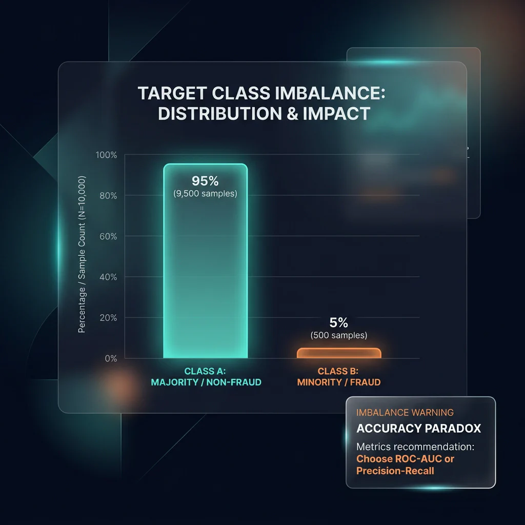
Target Class Imbalance - Describing feature scales and bounds using
Slide 20: Boxplots for Outlier Detection
Slide Title: Visualizing Outliers with Seaborn
Core Concepts:
- Outliers can heavily skew linear ML models (like Ordinary Least Squares).
- Anatomy of a boxplot: quartiles, whiskers, and outlier points (IQR method).
- Whisker Bounds: The whiskers extend to the minimum and maximum data points within the non-outlier limits (
Q1 - 1.5*IQRandQ3 + 1.5*IQR). - Using
sns.boxplot()orsns.violinplot()to inspect numerical feature ranges.
Python Implementation:
import seaborn as sns
import matplotlib.pyplot as plt

# Boxplot for Outlier Detection across Groups
sns.boxplot(
    data=df_ts,
    x='membership',
    y='amount',
    hue='is_fraud',
    palette='muted'
)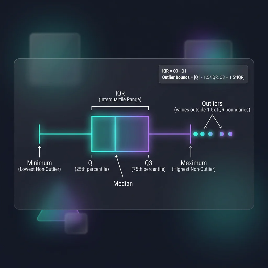
Outlier Boxplot
Slide 21: Correlation Matrices for Feature Selection
Slide Title: Multi-Collinearity: Correlation Heatmaps
Core Concepts:
- Multicollinearity (highly correlated features) destabilizes coefficients in linear models.
- Calculating Pearson correlation:
df.corr(numeric_only=True). - Visualizing relationships with Seaborn
sns.heatmap()to identify features to drop.
Python Implementation:
# Isolate numeric columns (excluding high-value flag)
numeric_cols = df_ts.select_dtypes(include=[np.number]).columns.tolist()
cols_to_corr = [col for col in numeric_cols if col not in ['is_high_value']]

# Pairwise correlation
corr_matrix = df_ts[cols_to_corr].corr()

# Draw correlation heatmap
sns.heatmap(corr_matrix, annot=True, cmap='coolwarm', fmt=".2f", linewidths=0.5)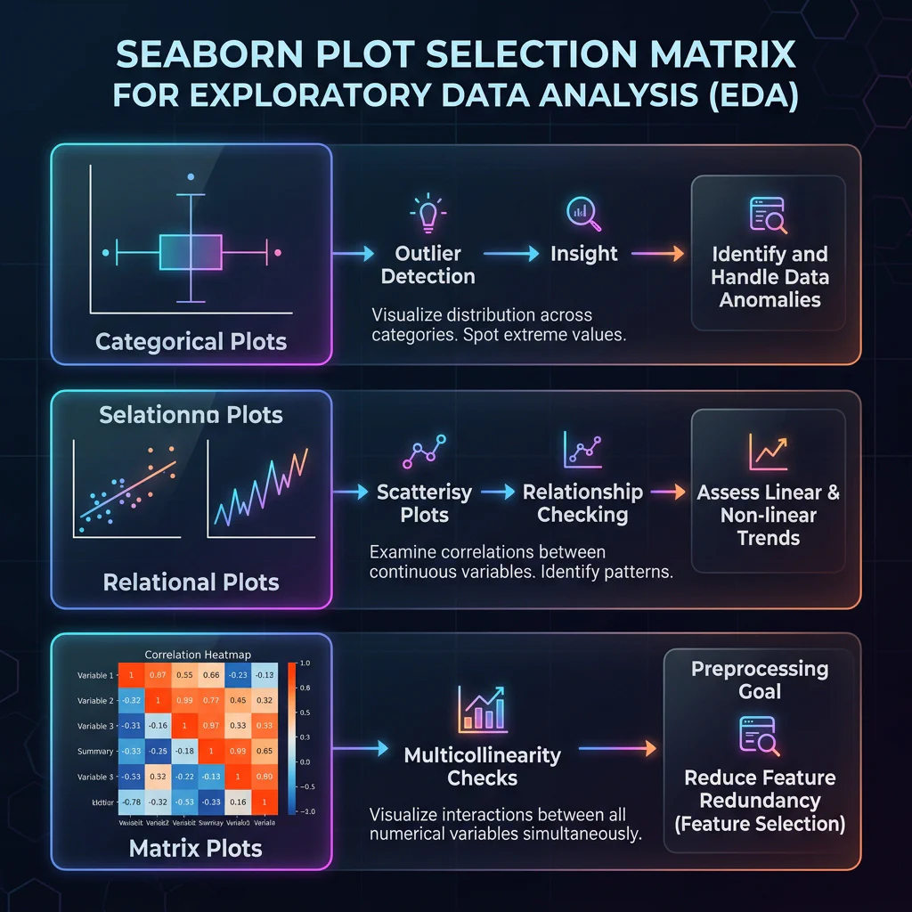
Seaborn Visualization Matrix Image
08. Recap & Scikit-Learn Handover (00:58 – 01:00)
Slide 22: ML Prep Checklist & Pandas 3.0 Roadmap
- Slide Title: Are You Ready for Scikit-Learn?
- Core Concepts:
- 5-Point Preprocessing Checklist: No NaNs, categories encoded, timestamps numerical, outliers checked, target $y$ split from features $X$.
- Pandas 3.0 Roadmap:
- PyArrow Backend by Default: Replaces NumPy for strings, leading to 10x faster string operations, lower memory footprints, and native missing value representation.
- Copy-on-Write (CoW): Active by default. Eliminates
SettingWithCopyWarningand avoids accidental deep copying of large arrays.
🧱 Appendix: Computer Architecture & Data Engineering 101
🧩 Cores vs. Threads: The Hardware Basics
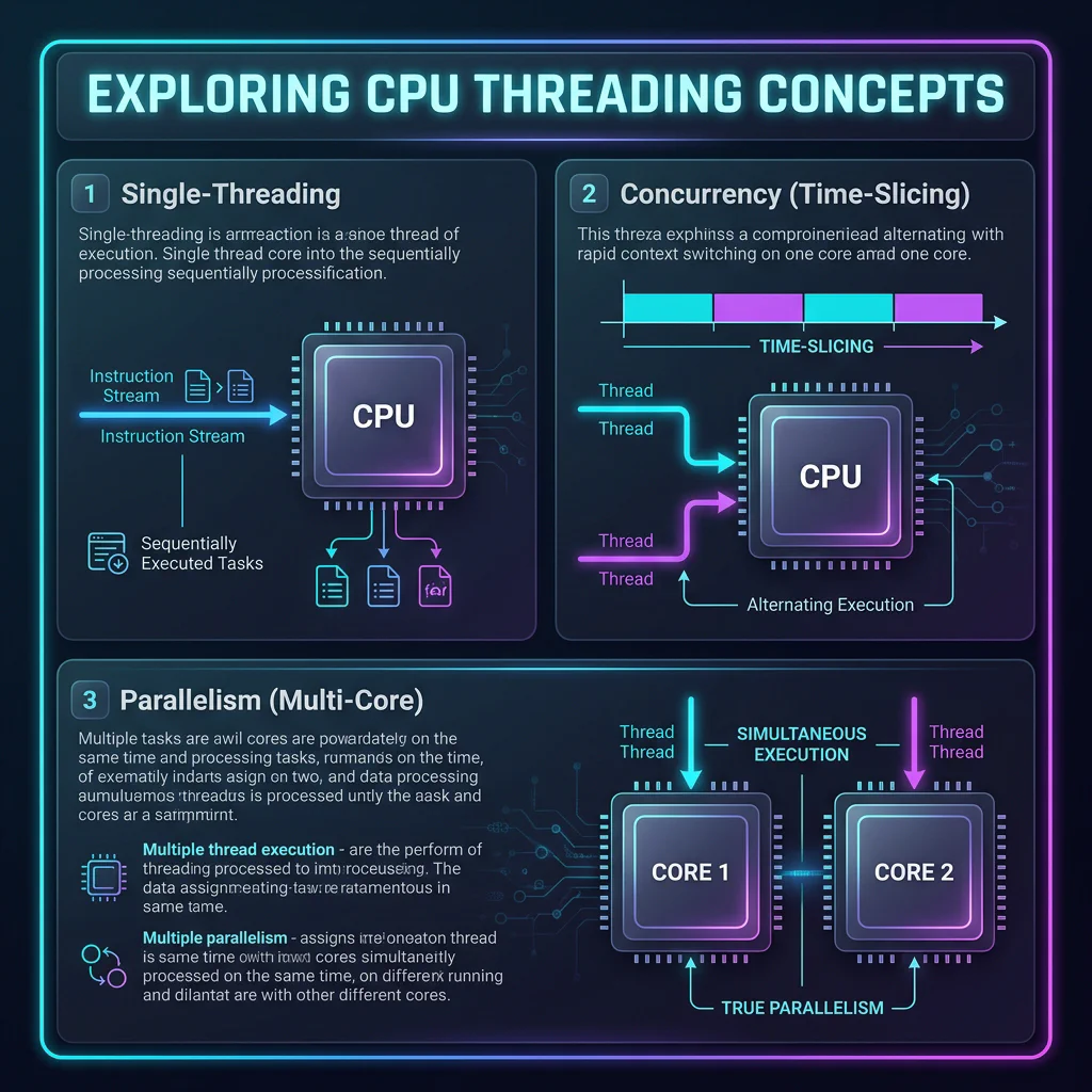
- Core: A physical, independent hardware processor inside the CPU that executes instructions.
- Thread: A virtual sequence of instructions executed by software.
🍽️ The Restaurant Analogy
| Concept | What It Is | Restaurant Analogy |
|---|---|---|
| Core | Physical hardware processor inside the CPU. | A physical chef working in the kitchen. |
| Thread | A stream of tasks executed by software. | A recipe/order ticket that needs to be prepared. |
| Single-Threading | One task is executed at a time. | One chef working on exactly one order from start to finish. |
| Multi-Threading | Multiple tasks are executed concurrently. | One chef juggling multiple orders (waiting for water to boil, etc). |
| Multi-Core Processing | Multiple physical processors execute tasks at the same time. | Multiple chefs working simultaneously on different orders. |
⚡ Cache Locality & SIMD (Desk Drawer vs. Library Warehouse)
- The Problem: If your data is scattered all over RAM (like a standard Python list containing object pointers), the CPU must fetch each element from slow RAM. This is called a Cache Miss.
- The Columnar Solution: If your data is stored in contiguous, aligned blocks of memory (like NumPy, Arrow, Polars, and DuckDB), the CPU fetches a whole chunk of data into L1 Cache once. It then uses SIMD (Single Instruction, Multiple Data) hardware registers to process multiple values in a single CPU cycle.
⏱️ The Latency Scale (Visualizing CPU Speeds)
If 1 CPU Cycle takes 1 second (equivalent to a human blink), the hardware operations scale as follows:
| Operation | Time in CPU Scale | Human Analogy |
|---|---|---|
| 1 CPU Cycle | 1 Second | A single blink of an eye. |
| L1 Cache Access | 0.5 Seconds | Grabbing a notebook on your desk. |
| L3 Cache Access | 15 Seconds | Grabbing a book from a nearby shelf. |
| Main Memory (RAM) | 2 Minutes | Walking down the hall to the water cooler. |
| Solid State Drive (SSD) | 2 Days | Taking a weekend trip to another city. |
| Mechanical Hard Drive (HDD) | 1.5 Months | Going on a long summer vacation. |
| Network Call (Internet) | 2 Years | Going to university and earning a degree. |
Data Engineering Rule of Thumb: Always optimize to minimize Network Calls and Disk Reads first. A single network query or reading from disk dominates your performance bottleneck, regardless of how fast your CPU code is.