We are excited to share the materials for our interactive conceptual masterclass: Introduction to Machine Learning & Modelling Techniques (Supervised, Unsupervised & Reinforcement Learning).
This session was designed specifically for beginner-to-intermediate data professionals to build a clear, visual, and practical mental map of machine learning paradigms and algorithms.
🚀 Presentation Resources
Session Outline & Content Blueprint
Below is the complete lesson blueprint and scheduling outline for the session.
Target Audience: Beginner-to-Intermediate Data Professionals
Format: 1-Hour Live Session (Interactive Presentation + Conceptual Walkthroughs)
Deliverable: Comprehensive, presentation-ready lesson outline with slide structures, talking points, concrete examples, and visual aids.
💡 How to Make This Session Highly Engaging & Interactive
To keep beginner-to-intermediate professionals hooked, use these five live engagement strategies:
- Interactive “Human-ML” Opener (2 mins): Before introducing definitions, show a slide with inputs (e.g., $X=[2, 4, 6]$) and outputs (e.g., $Y=[4, 8, 12]$) and ask the chat to “train” themselves to find the rule. This illustrates learning from scratch.
- Interactive Concept Quizzes: Three dedicated slides to rapid-fire conceptual testing covering (1) Classification vs. Regression, (2) Clustering vs. Dimensionality Reduction, and (3) Supervised vs. Unsupervised vs. Reinforcement Learning.
- Spot-the-Outlier Clustering: Show the clustering diagram and ask the audience to write the coordinates of anomalous data points in the chat.
- Interactive Maze Storytelling (Reinforcement Learning): Walk through the robot maze step-by-step, asking the audience: “If the robot steps on the fire hazard, what reward should we give it?” to build the intuition of reinforcement learning before showing the success slide.
- No-Code Tool Matchmaker: Display a list of problems at the end, and have the audience match them to the correct Python library (
pandasvs.scikit-learnvs.pytorch).
⏱️ 60-Minute Block Schedule
| Time | Slide Range | Block Name | Focus | Key Deliverables & Interactive Elements |
|---|---|---|---|---|
| 00:00 – 00:08 | Slides 1 – 3 | 01. Session Kickoff & The ML Landscape | AI, ML, DL, and LLMs | Venn diagram, “Learn from scratch,” paradigm mapping |
| 00:08 – 00:25 | Slides 4 – 13 | 02. Supervised Learning & Model Performance | Regression, Regularization, Classification, Ensembles | Overfitting/Underfitting, OLS Math, Ridge/Lasso cost, Code snippets |
| 00:25 – 00:30 | Slide 14 | 03. Supervised Concept Quiz | Classification vs. Regression | 4 live practice scenarios to test comprehension |
| 00:30 – 00:43 | Slides 15 – 19 | 04. Unsupervised Learning Deep Dive | Clustering & Dimensionality Reduction | Spot-the-outlier, KMeans vs DBSCAN comparison, PCA projections |
| 00:43 – 00:48 | Slide 20 | 05. Unsupervised Concept Quiz | Clustering vs. Dim. Reduction | 3 live practice scenarios to test comprehension |
| 00:48 – 00:50 | Slide 21 | 06. Unsupervised Case Studies | Unsupervised Applications | 3 real-world case studies (cohorts, genomics, anomalies) |
| 00:50 – 00:55 | Slides 22 – 25 | 07. Reinforcement Learning Overview | Trial-and-Error Learning | Interactive robot maze walkthrough, Q-learning, policy gradients |
| 00:55 – 00:58 | Slides 26 – 30 | 08. Model Taxonomy, Selection & Live Demos | Model Selection, Families, Workflow, Demos | Decision grid, 5 Families, 6-Step Workflow timeline, Live Demo templates |
| 00:58 – 01:00 | Slides 31 – 36 | 09. Recap, Quiz & Live Q&A | Review & Open Discussion | Tooling map, key takeaways, visual cheatsheet, paradigm matchmaker quiz, audience Q&A |
01. Session Kickoff & The ML Landscape (00:00 – 00:08)
Slide 1: Welcome & Session Overview
Slide Title: Demystifying Machine Learning: From Scratch to Actionable Models
Core Concepts:
- Basics of machine learning: rules-based programming vs. learning patterns.
- Learning from scratch: models as mathematical approximations of historical datasets.
- Essential terminology: features (inputs), targets (outputs), parameters, predictions.

Machine Learning Cover Graphic
Slide 2: Mapping the Landscape: AI vs. ML vs. DL vs. LLM
Slide Title: Navigating the AI Ecosystem
Core Concepts:
- Artificial Intelligence (AI): Overton field of machines mimicking human intelligence.
- Machine Learning (ML): Algorithmic subset learning rules directly from data.
- Deep Learning (DL): Nested neural network layers modeling raw unstructured data.
- Large Language Models (LLM): Transformer architectures mapping sequences of human language.

AI vs ML vs DL vs LLM Venn Diagram
Slide 3: The Three Pillars of ML (Plain English Definitions)
Slide Title: The Three Pillars of Machine Learning
Core Concepts:
- Supervised Learning: Learning with a teacher (predicting labels using labeled historical datasets).
- Example: Predicting customer default risk using credit details.
- Unsupervised Learning: Self-discovery (identifying hidden structures or patterns in unlabeled data).
- Example: Segmenting buyers into shopping cohorts.
- Reinforcement Learning: Trial and error (an agent maximizing rewards through environment actions).
- Example: Training a robot vacuum to navigate around hazards.
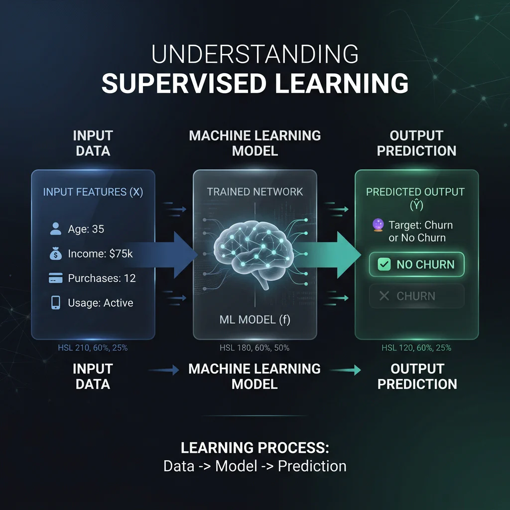
Supervised Learning Pipeline - Supervised Learning: Learning with a teacher (predicting labels using labeled historical datasets).
02. Supervised Learning & Model Performance (00:08 – 00:25)
Slide 4: Machine Learning Terminology Foundations
- Slide Title: Machine Learning Terminology
- Core Concepts:
- The Core Learning Frameworks: Supervised Learning (labeled inputs), Unsupervised Learning (unlabeled patterns), Reinforcement Learning (reward loop), and Semi-Supervised Learning (cost-effective mix).
- The Mechanics of Learning:
- Features & Target: Features (independent variables
X) vs. Target (dependent predictionY). - Loss & Cost Function: Measures error magnitude; minimized during training.
- Gradient Descent & Learning Rate: Weight optimizer and its step-size hyperparameter.
- Parametric vs. Non-Parametric: Fixed complexity weights (Linear Regression) vs. growing structural complexity (k-NN, Decision Trees).
- Linear vs. Non-Linear vs. Spatial: Straight lines vs. curved bounds vs. coordinate proximity.
- Features & Target: Features (independent variables
- Generalisation & Pitfalls: Overfitting (noise memorization) vs. Underfitting (too rigid), Bias-Variance Tradeoff (balancing simplicity and sensitivity), and Regularisation (L1 Lasso / L2 Ridge complexity penalties).
- Data Splitting & Evaluation:
- Splits: Train (teaches weights), Validation (tunes hyperparameters), Test (hidden final holdout).
- Cross-Validation: Rotating chunks to prevent lucky splits.
- Confusion Matrix: Layout mapping TP, TN, FP, FN classification coordinates.
- Precision vs. Recall: Positive prediction accuracy vs. sensitivity to positive cases.
Slide 5: Introduction to Supervised Learning
Slide Title: Supervised Learning: Predicting Target Outputs
Core Concepts:
- Learning a mapping function $Y = f(X)$ where $X$ represents inputs and $Y$ represents outputs.
- Regression: Output is a continuous numerical value.
- Example: Estimating real estate market prices.
- Classification: Output is a discrete categorical label.
- Example: Flagging spam emails.
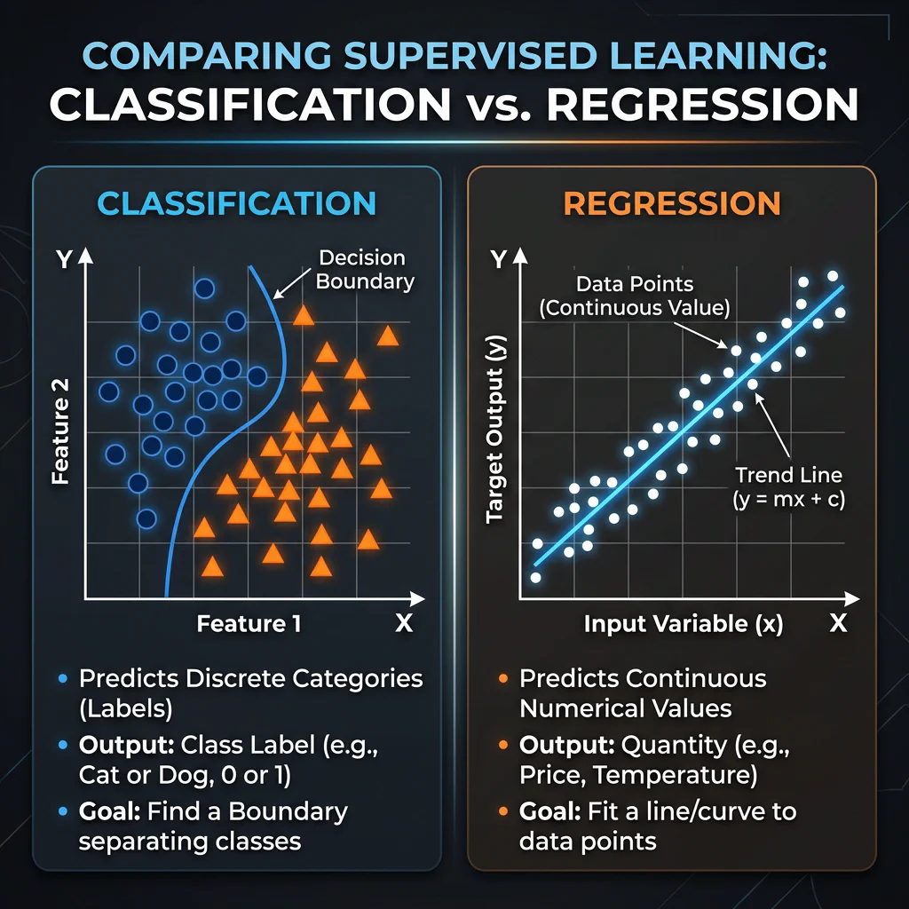
Classification vs Regression Plot
Slide 6: Model Performance: Overfitting, Bias & Tuning
Slide Title: Model Performance: Overfitting, Bias & Tuning
Core Concepts:
- Underfitting (High Bias): Model is too simple to capture trends.
- Example: Predicting house price using only size, ignoring location.
- Overfitting (High Variance): Model memorizes training noise; fails to generalize.
- Example: Fitting a high-degree polynomial that matches outliers but fails on new data.
- Cross-Validation: Splitting data into $k$-folds to validate generalized accuracy.
- Example: Splitting data into 5 groups, training on 4, validating on 1, rotating 5 times.
- Hyperparameters: Structural choices tuned to control complexity.
- Example: Restricting a decision tree’s depth to 3 levels, or setting $k=5$ neighbors.
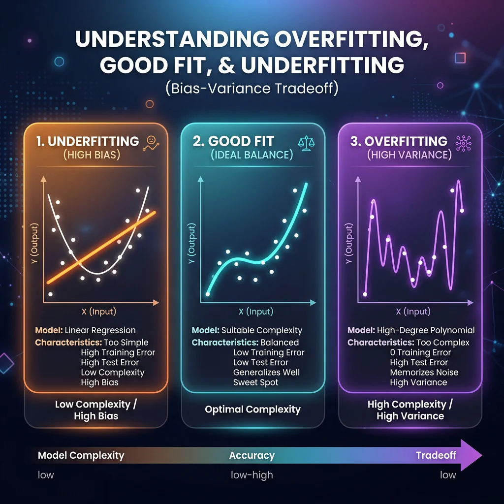
Bias-Variance Trade-off Plot - Underfitting (High Bias): Model is too simple to capture trends.
Slide 7: Regression Models In-Depth
- Slide Title: Regression: Predicting Continuous Numbers
- Core Concepts:
- Linear Regression: Fits a straight line minimizing residual sum of squares.
- Regularization (Ridge & Lasso): Limits coefficient size using budget penalties.
- Ridge vs. Lasso: Ridge shrinks weights evenly; Lasso drives some coefficients completely to zero (automated feature selection).
- Selection Guide:
- Linear Regression: Choose for simple, linear trends where coefficient interpretability is paramount.
- Ridge (L2): Choose to handle multicollinearity (highly correlated features) while keeping all features.
- Lasso (L1): Choose to perform automated feature selection and create sparse, highly interpretable models.
Slide 8: Mathematical OLS (Linear Regression)
Slide Title: Ordinary Least Squares (OLS)
Mathematical Presentation:
- Linear Equation: $y = \beta_0 + \beta_1 x_1 + \dots + \beta_n x_n$
- Cost Function: $MSE = \frac{1}{n} \sum (y_i - \hat{y}_i)^2$
Conceptual Example:
- Predicting housing price ($y$) using size ($x_1$). Intercept $\beta_0$ represents base land price, and weight $\beta_1$ is cost per sq ft.
Python Implementation:
from sklearn.linear_model import LinearRegression
model = LinearRegression(fit_intercept=True)
model.fit(X_train, y_train)
OLS Linear Regression trend line and coordinates
Slide 9: Regularization Mathematics (L1 vs. L2 Penalty)
Slide Title: Regularization Math
Mathematical Presentation:
- Ridge (L2 Penalty): $J(w) = MSE + \alpha \sum (w_j)^2$
- Lasso (L1 Penalty): $J(w) = MSE + \alpha \sum |w_j|$
Weight Shrinkage Example:
- High penalty $\alpha$ shrinks weights. Ridge (L2) scales all features down evenly, while Lasso (L1) zeros out less important features (e.g. wall color), acting as feature selector.
Python Implementation:
from sklearn.linear_model import Ridge, Lasso
ridge = Ridge(alpha=1.0)
lasso = Lasso(alpha=0.1)
Bias Variance tradeoff: Underfitting vs Good Fit vs Overfitting
Slide 10: Classification: Part 1 (Linear & Non-Linear)
Slide Title: Classification: Categorizing Data Points
Core Concepts:
- Logistic Regression: Outputs binary category probabilities via a sigmoid curve (e.g. loan defaults).
- Support Vector Machines (SVM): Solves boundaries by maximizing margins separating groups (e.g. OCR letter reading).
- Selection Guide:
- Logistic Regression: Choose if you need fast training, highly interpretable coefficients, or explicitly require the probability of an outcome.
- SVM: Choose if data is not linearly separable (using kernels), features exceed samples, or maximum accuracy is needed without probability mapping.
- k-NN: Choose if the dataset is small, the decision boundaries are highly irregular/non-linear, and you need a simple instance-based baseline with no training phase.
- Hyperparameter C: In both Logistic Regression and SVM, the C parameter controls regularization strength. A smaller C increases regularization (prevents overfitting by keeping weights small), while a larger C fits training data perfectly.
Python Implementation:
from sklearn.linear_model import LogisticRegression
from sklearn.svm import SVC
lr = LogisticRegression(C=1.0)
svm = SVC(kernel='rbf', C=1.0)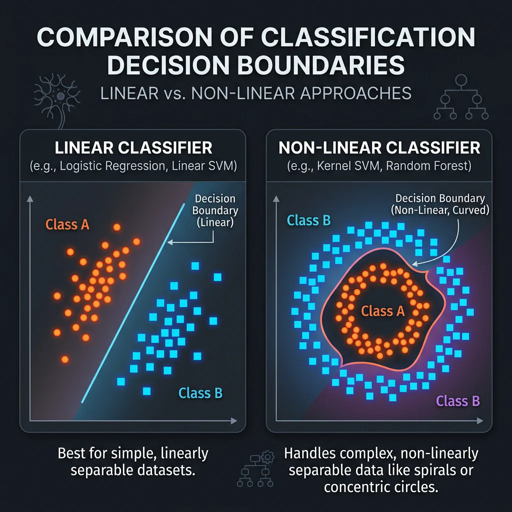
Classification Decision Boundaries
Slide 11: Distance-Based: k-NN
Slide Title: Distance & Spatial Closeness: k-NN
Core Concepts:
- Classifies a target point based on a majority vote of its $k$-closest spatial neighbors.
- Hotel Example: Classify a hotel as Budget Hostel vs. Luxury Resort using Price per Night ($) and Distance to Beach (meters) spatial coordinates under $k=5$.
Python Implementation:
from sklearn.neighbors import KNeighborsClassifier
knn = KNeighborsClassifier(n_neighbors=5, p=2)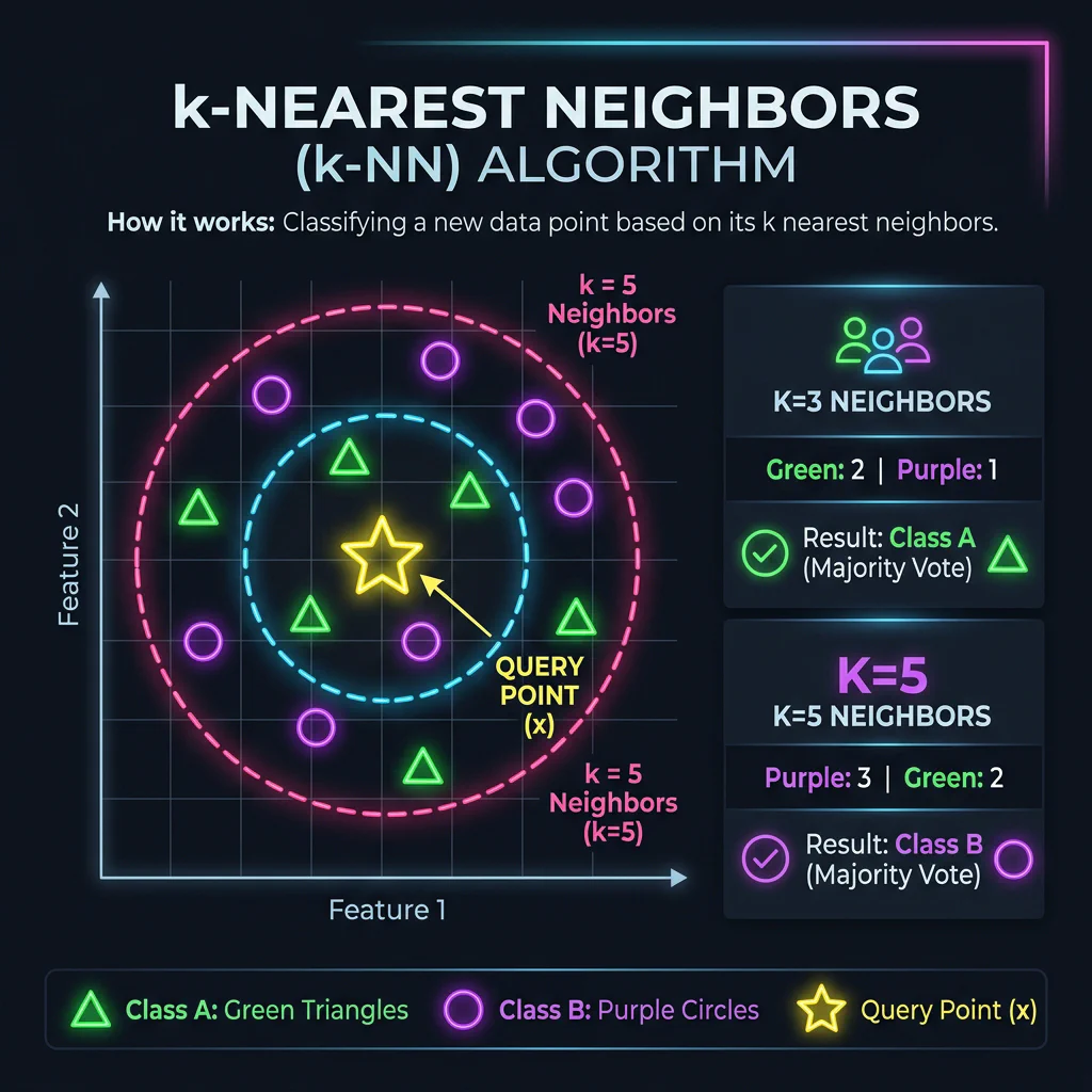
k-NN Voting Circles
Slide 12: k-NN Classification: Step-by-Step
- Slide Title: k-NN: Step-by-Step Example
- Core Concepts:
- Step 1: Distance Measurement: Compute Euclidean distance to all known points from query coordinate (6,4).
- Step 2: Sorting & Nearest Neighbors: Find the 3 points with the smallest distance.
- Step 3: Majority Vote: Tallies the classes of the 3 neighbors to make the final prediction (Orange).
Slide 13: Tree-Based Supervised Models Deep Dive
Slide Title: Tree Models: From Single Decisions to Advanced Ensembles
Core Concepts:
- Decision Trees: Splits features progressively using binary rules.
- Loan Default Example: Split first on Credit Score > 650, then on Debt-to-Income (DTI) < 40%.
- Random Forests (Bagging): Combines independent trees in parallel to reduce variance.
- XGBoost (Boosting): Fits sequential trees correcting residual errors of past trees.
- Selection Guide:
- Decision Trees: Choose if you need simple, visual, rules-based logic with zero data scaling that is easily explainable to non-technical users.
- Random Forest: Choose for high accuracy out-of-the-box, resistance to overfitting, and a robust model with minimal tuning.
- XGBoost: Choose when competing for maximum accuracy on structured tabular data, having compute power, and requiring fine-grained tuning.
- Decision Trees: Splits features progressively using binary rules.
Python Implementation:
from sklearn.ensemble import RandomForestClassifier
from xgboost import XGBClassifier
rf = RandomForestClassifier(n_estimators=100, max_depth=8)
xgb = XGBClassifier(n_estimators=100, learning_rate=0.1)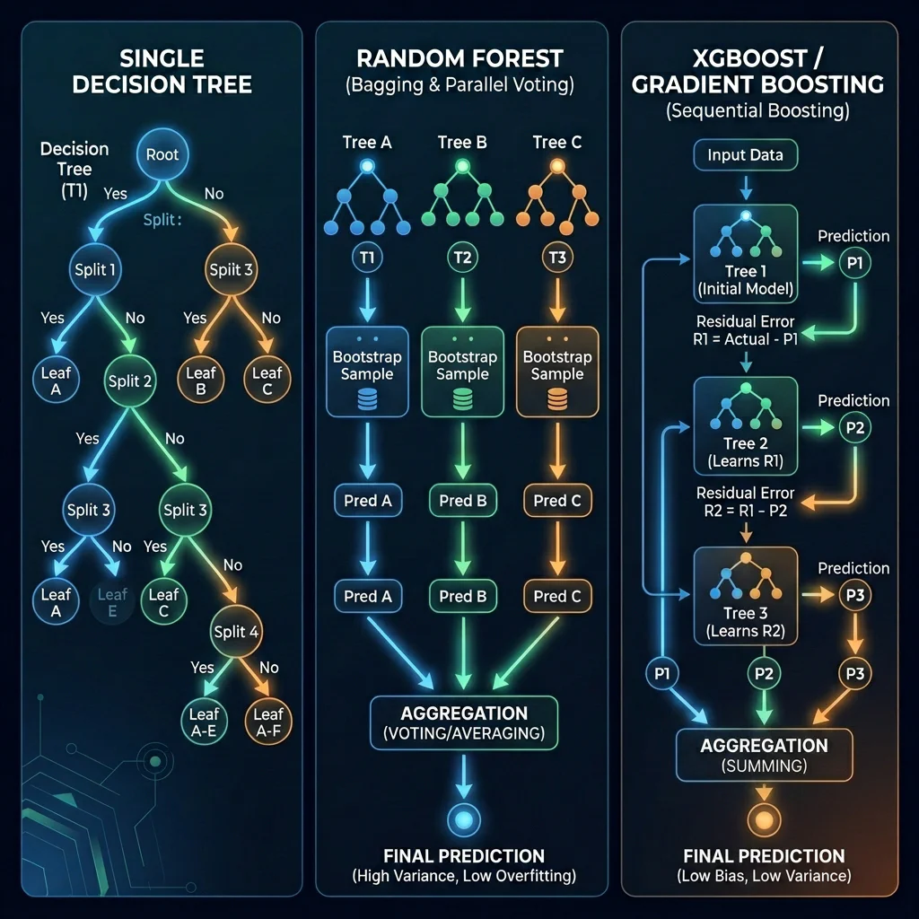
Tree Models Comparison
Slide 14: Supervised Learning Case Studies
- Slide Title: Supervised Learning: Case Studies
- Key Scenarios:
- Telecom customer churn (Classification using XGBoost).
- Real estate pricing (Regression using Ridge/Lasso).
- Email spam classification (Classification using Naive Bayes/SVM).
03. Supervised Concept Quiz (00:25 – 00:30)
Slide 15: Live Quiz: Classification vs. Regression Scenarios
- Slide Title: Test Your Knowledge: Which Paradigm Fits?
- Scenarios Covered:
- Stock price prediction tomorrow (Regression).
- Phishing email check (Classification).
- Delivery duration ETA (Regression).
- Medical tumor classification (Classification).
04. Unsupervised Learning Deep Dive (00:30 – 00:43)
Slide 16: Introduction to Unsupervised Learning
- Slide Title: Unsupervised Learning Basics
- Core Concepts:
- Discovering structures in unlabeled tables.
- Sub-types: Clustering, Dimensionality Reduction, Anomaly Detection.
Slide 17: Clustering Techniques In-Depth
- Slide Title: Clustering Algorithms
- Core Concepts:
- K-Means: Groups data around $k$ centroids by minimizing Euclidean distance to central averages. Assumes spherical clusters, failing completely on circular tracks or rings.
- Hierarchical Clustering: Agglomerative grouping based on local proximities, building a tree structure (dendrogram).
- Distance Metric Clarification: It uses distance measures like Euclidean distance.
- Distance Usage Difference: K-Means uses Euclidean distance to measure proximity to global central centroids; Hierarchical uses it to measure local pairwise distances between points/groups.
- Linkage Criteria: Single Linkage (nearest points) measures distance between the closest points of separate clusters. Like DBSCAN, it creates a chaining effect to trace circular rings and arbitrary shapes. Complete Linkage (furthest points) & Ward’s Method (minimize variance) force compact spherical clusters, behaving like K-Means.
- Selection Guide:
- K-Means: Choose for spherical clusters of similar size, and when speed and scalability on large datasets are required.
- Hierarchical: Choose if you need to inspect a tree hierarchy (dendrogram) to decide cluster count, or require deterministic results on small-to-medium datasets.
- DBSCAN: Choose for arbitrary/non-spherical shapes (loops, rings), when noise/outliers need filtering, and cluster count k is unknown.
- DBSCAN: Density-based scanning using radius connectivity to trace arbitrary shapes organically and isolate noise.
- Shape Discovery & Local Scanning: Uses local radius scans (
eps) around individual points rather than a global centroid. Points within each other’s radius connect like chain links (chain-linking effect), allowing the cluster to grow organically in any direction. - Key Parameters: Eps (Radius) and MinPts / MinSamples.
- Shape Discovery & Local Scanning: Uses local radius scans (
- Python Implementation:
from sklearn.cluster import KMeans, DBSCAN kmeans = KMeans(n_clusters=3, random_state=42) dbscan = DBSCAN(eps=0.5, min_samples=5) - Visual Aids:
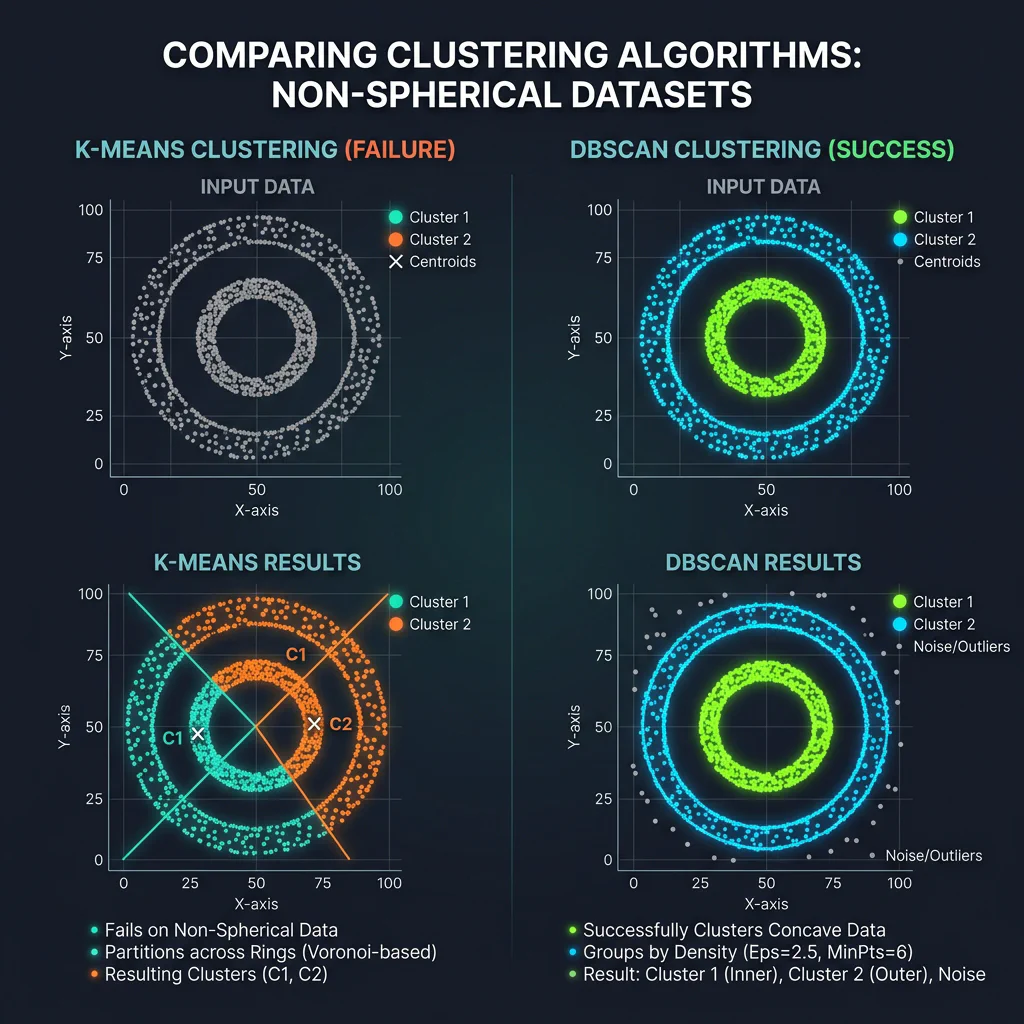
K-Means vs DBSCAN Comparison 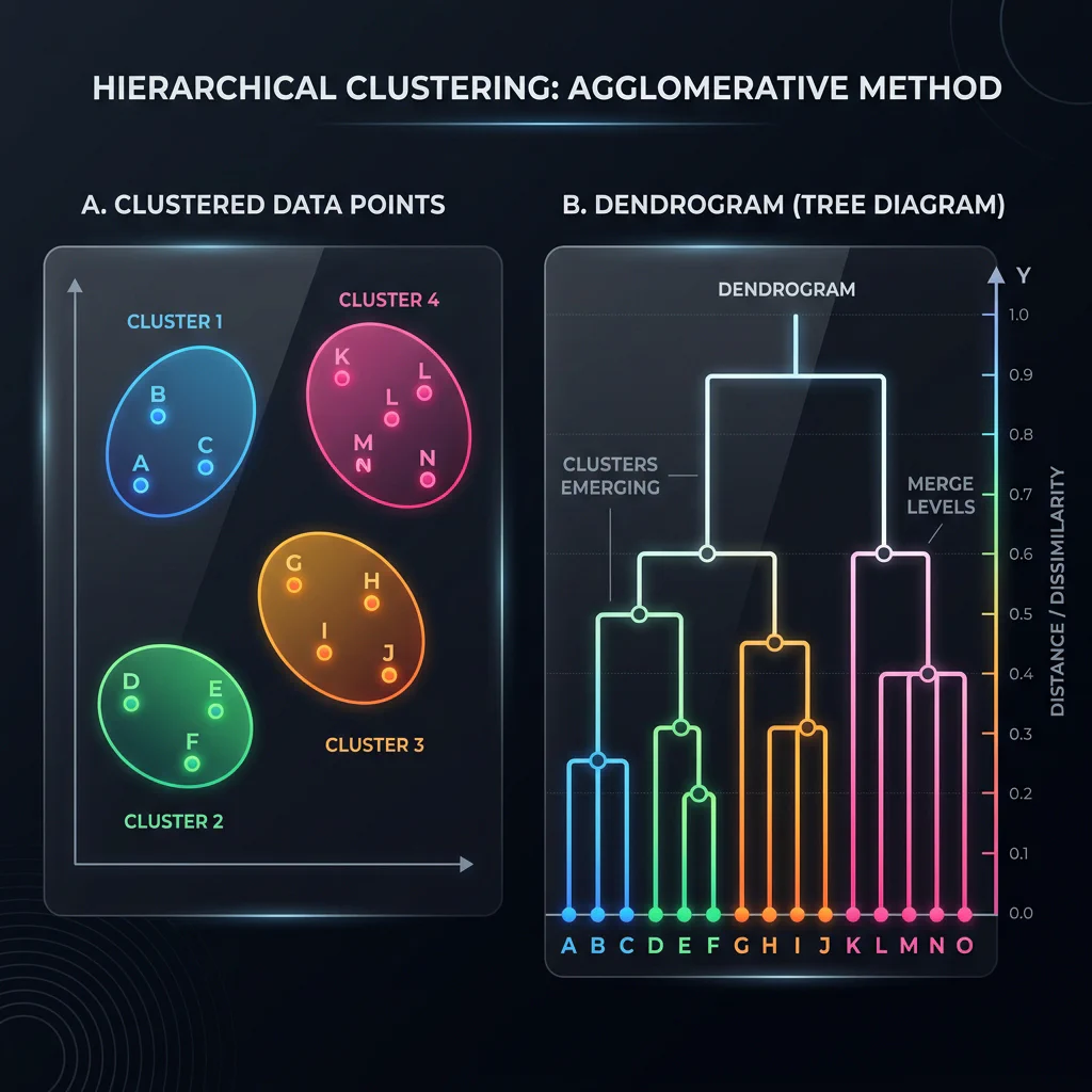
Dendrogram
Slide 18: Mechanics of Clustering: How They Work
- Slide Title: Mechanics of Clustering: How They Work
- Core Concepts:
- K-Means Mechanism: Centroid initialization (Initialize), distance-based mapping (Assign), mean coordinate update (Update), and mathematical iteration (Iterate) to convergence.
- Hierarchical Mechanism: Bottom-up agglomerative single-element clusters (Initialize), distance/linkage matrix scans (Measure), progressive parent cluster merges (Merge), and dendrogram logging (Iterate).
- DBSCAN Mechanism: Epsilon-neighborhood scans (Scan Neighbors), Core Point thresholds (Core Points), Border Point clustering extensions (Expand Border), and outliers noise identification (Isolate Noise).
Slide 19: K-Means Clustering: Step-by-Step
- Slide Title: K-Means: Step-by-Step Example
- Core Concepts:
- Step 1: Distance Assignment: Calculate distance from customers User A-D to centroids C1(20,3) and C2(40,8), and assign them to the closest one.
- Step 2: Centroid Updating: Compute the mean coordinate of assigned users for C1 and C2 to obtain new centers.
- Step 3: Convergence: Iterates until centroids no longer change coordinate positions.
Slide 20: Dimensionality Reduction Concepts
- Slide Title: Dimensionality Reduction
- Core Concepts:
- PCA: Projects variables orthogonally to maximize variance compression.
- t-SNE: Maps complex manifolds locally to visual 2D/3D distributions.
- Selection Guide:
- PCA: Choose for fast, linear noise reduction and feature compression prior to downstream modeling while preserving global variance.
- t-SNE & UMAP: Choose strictly for 2D/3D visualization of complex, non-linear manifolds, preserving local neighborhoods to identify visible subgroups.
- Python Implementation:
from sklearn.decomposition import PCA from sklearn.manifold import TSNE pca = PCA(n_components=2) tsne = TSNE(n_components=2, perplexity=30) - Visual Aids:
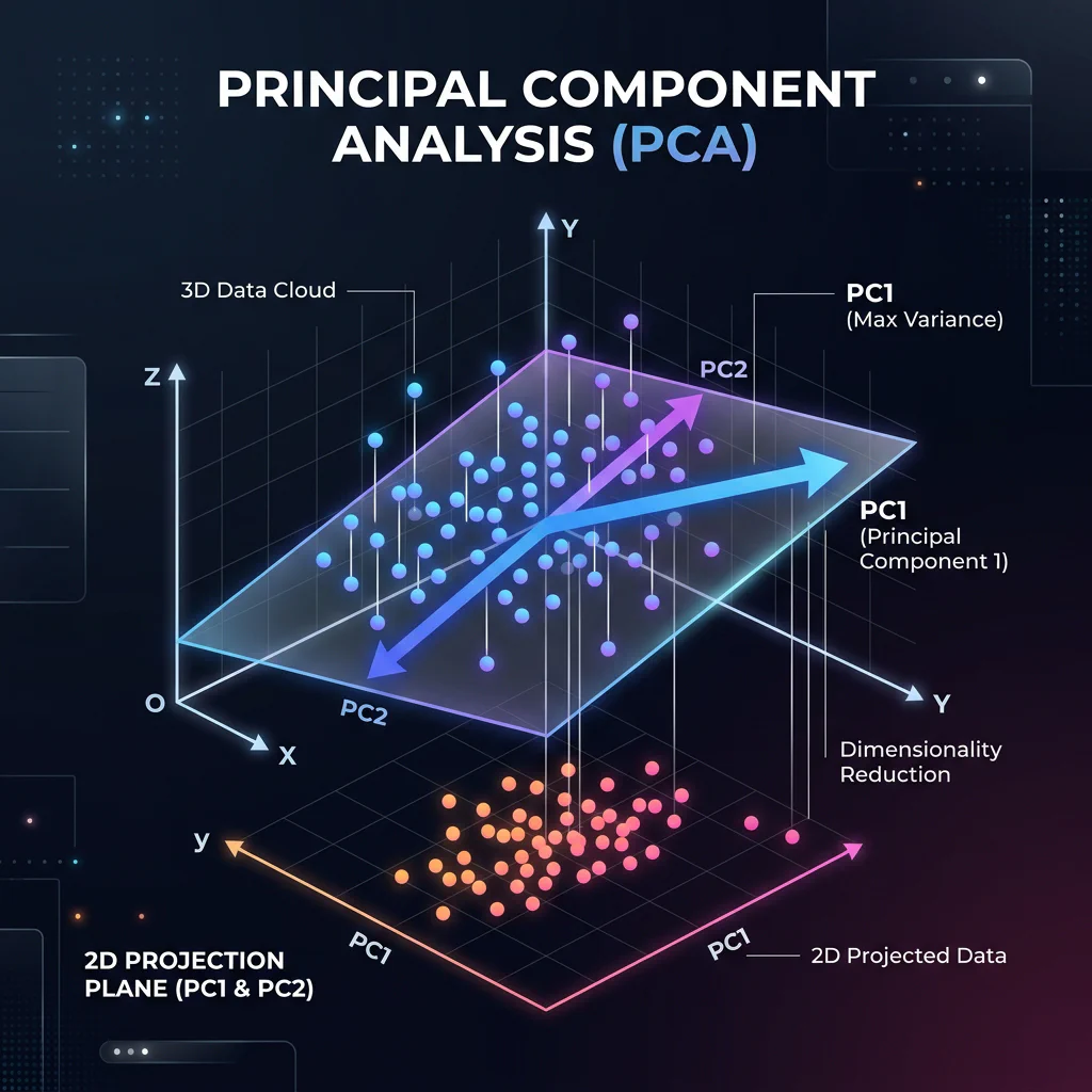
PCA Projection 3D to 2D 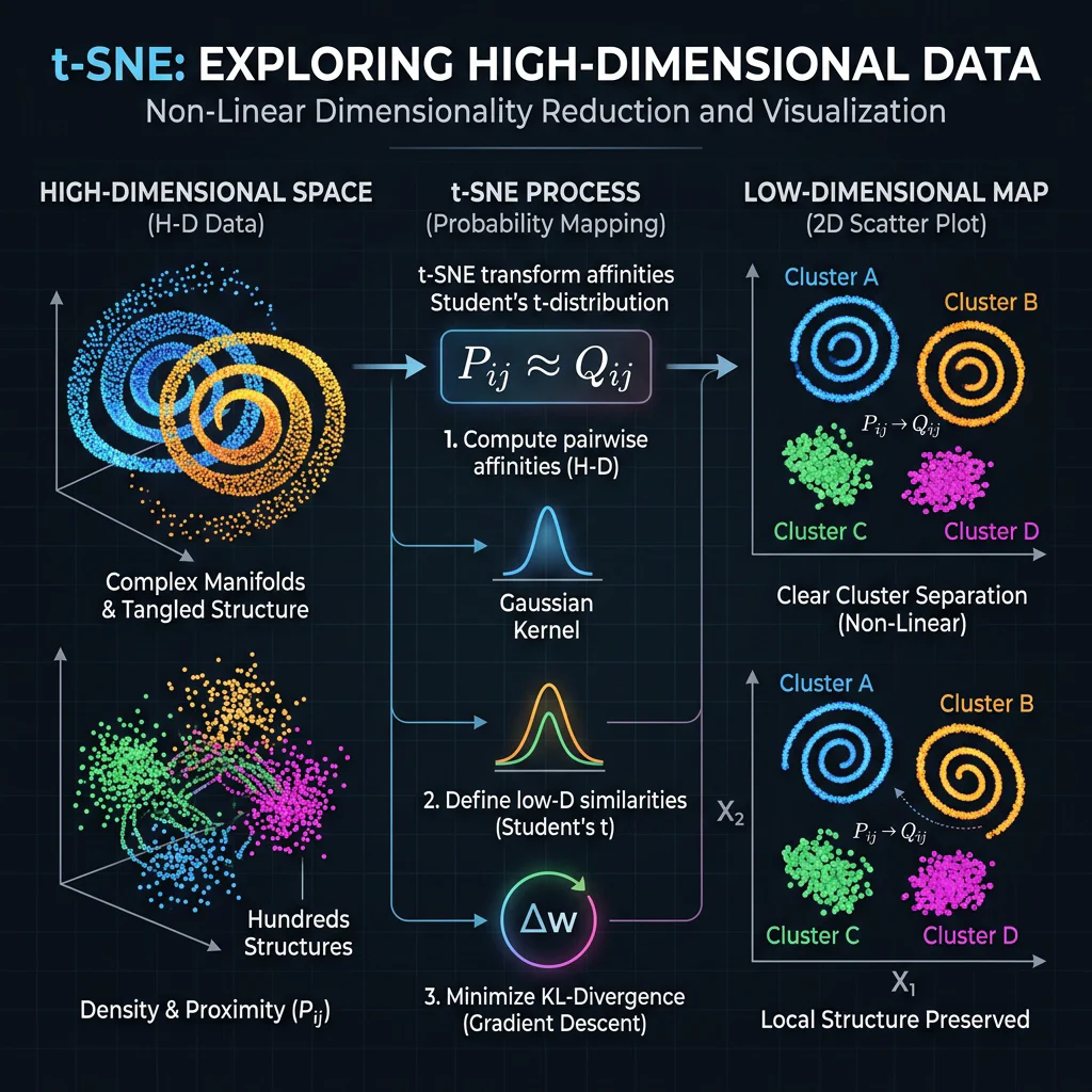
t-SNE Embeddings Mapping
05. Unsupervised Concept Quiz (00:43 – 00:48)
Slide 21: Unsupervised Quiz: Clustering or Dimensionality Reduction?
- Slide Title: Test Your Knowledge: Clustering or Dimensionality Reduction?
- Scenarios Covered:
- Group delivery drops coordinates (Clustering).
- Compress 50 survey columns into 3 coordinates (Dimensionality Reduction).
- Segment news articles into topics folders (Clustering).
06. Unsupervised Case Studies (00:48 – 00:50)
Slide 22: Unsupervised Learning – Example Problems & Model Usage
- Slide Title: Unsupervised Learning in Practice: 3 Case Studies
- Key Scenarios:
- E-commerce customer cohort segmentation (KMeans).
- High-dimensional patient genomics visualization (t-SNE).
- Bank transactions fraud anomaly detection (Isolation Forest).
07. Reinforcement Learning Overview (00:50 – 00:55)
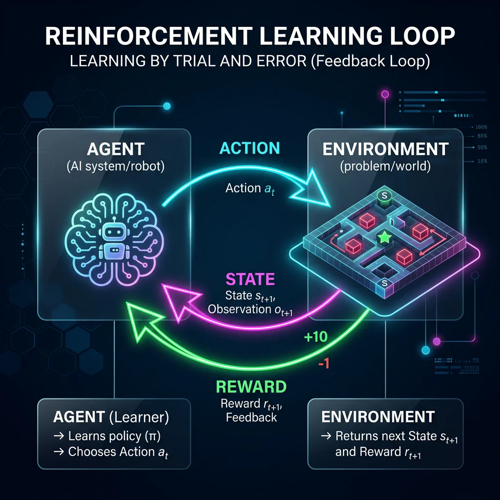
Slide 23: Introduction to Reinforcement Learning
Slide Title: Reinforcement Learning: Learning by Trial and Error
Core Concepts:
- Five elements: Agent, Environment, State, Action, Reward.
Reinforcement Learning Loop
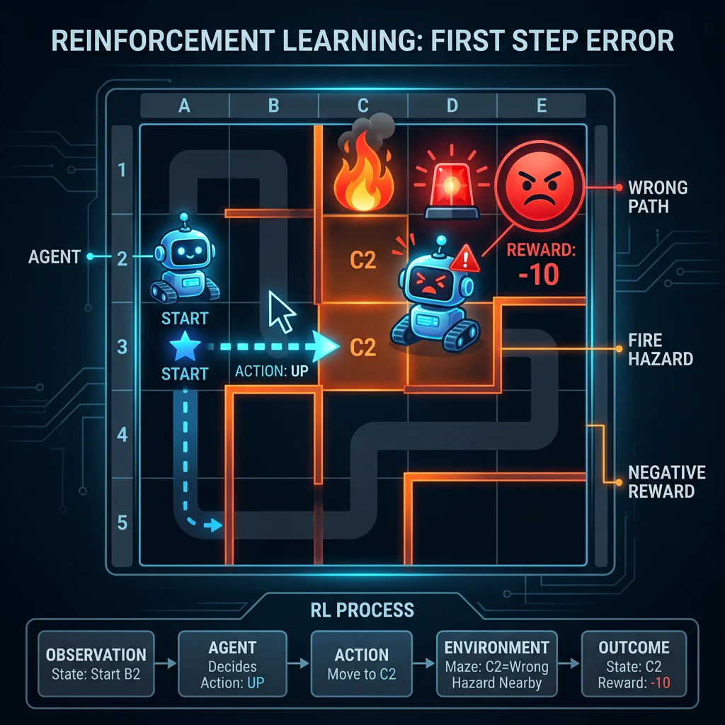
Slide 24: The Learning Journey of an Agent (Visual Walkthrough)
Slide Title: Interactive: RL Agent Learning Journey
Core Concepts:
- Step 1: Blind exploration yields a hazard penalty (fire).
- Step 2: Policy correction finds the reward path (battery charger).
Step 1: Fail 
Step 2: Success
Slide 25: Core RL Concepts & Algorithms
- Slide Title: RL Core Concepts & Algorithms
- Core Concepts:
- Exploration vs. Exploitation balance.
- Q-Learning (Value-based): expected reward index mapping.
- Policy Gradients (Policy-based): direct probability distribution scaling.
- Python Implementation:
# Q-learning setup
import gymnasium as gym
env = gym.make('FrozenLake-v1')

# Policy Gradient (PPO) model
from stable_baselines3 import PPO
model = PPO('MlpPolicy', env)
Slide 26: Reinforcement Learning Case Studies
- Slide Title: Reinforcement Learning Case Studies
- Key Scenarios:
- Game-playing bot calibrations (Deep Q-Networks / DQN).
- Robotic arm item grasp (PPO / continuous control).
- Dynamic ad bidding (Thompson Sampling / Multi-Armed Bandits).
08. Model Taxonomy, Selection & Live Demos (00:55 – 00:58)
Slide 27: Choosing the Right Model: Decision Matrix
- Slide Title: Choosing the Right Model: Decision Matrix
- Key Concepts:
- Supervised Selection: Linear Regression (interpretable baseline), Ridge/Lasso (regularization), Logistic Regression (binary baseline), SVM (margins), Ensembles (Random Forest/XGBoost for tabular complexity).
- Unsupervised Selection: KMeans (spherical cohorts), Hierarchical (taxonomic dendrograms), DBSCAN (arbitrary density, noise exclusion), PCA (downstream speedup), t-SNE (2D/3D visualization only).
- Reinforcement Selection: Bandits (explore/exploit feedback loop), Q-Learning (discrete low-dimension matrix grids), Policy Gradients/PPO (continuous continuous mechanics).
Slide 28: How Many Machine Learning Models Are There?
Slide Title: Mapping the Model Space: Five Core Families
Five Families: Linear Models, Tree-Based Ensembles, Distance-Based Spatial, Probabilistic, Neural Networks.
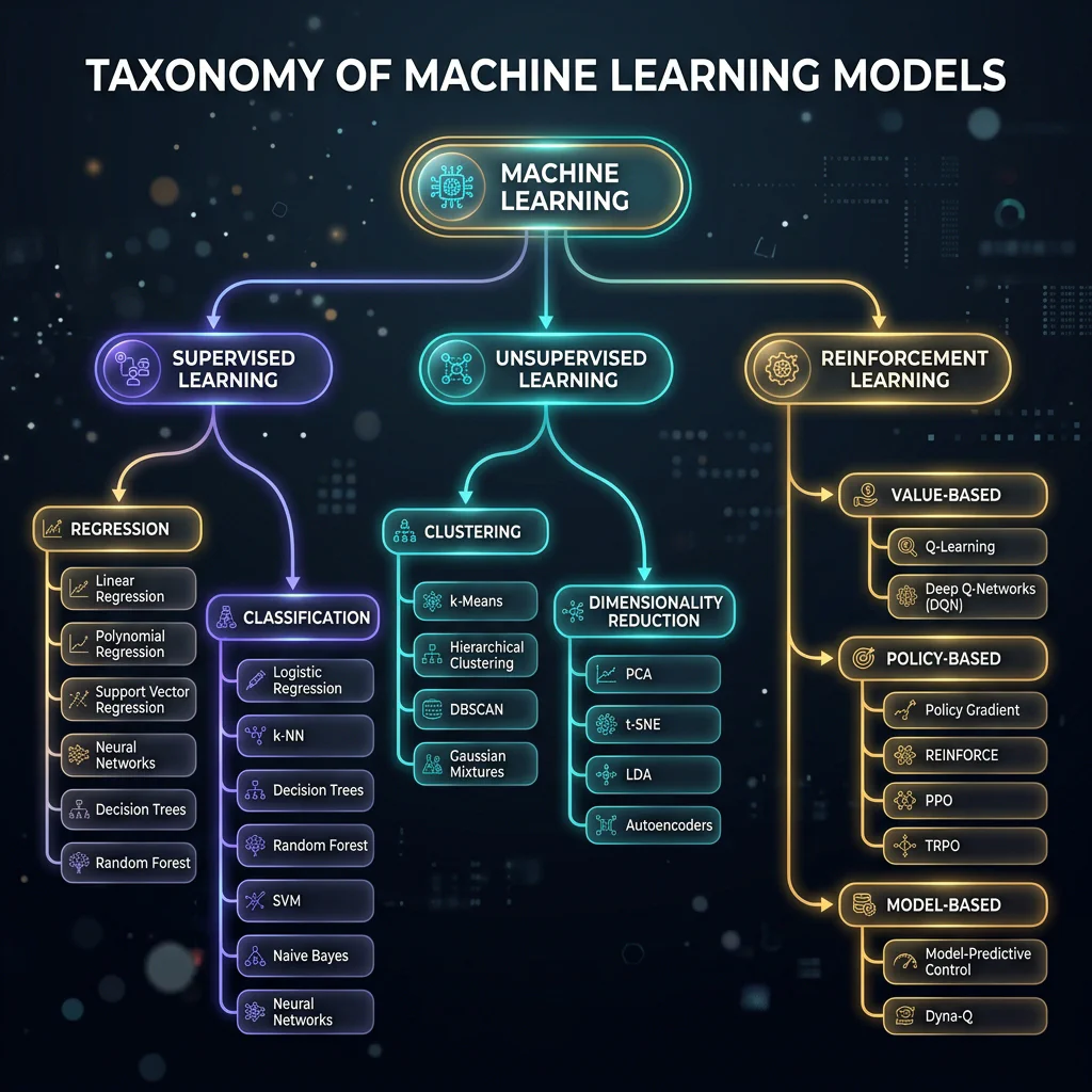
Model Taxonomy Tree Diagram
Slide 29: The End-to-End ML Pipeline
Slide Title: The 6-Step Machine Learning Workflow
Six Steps: Data Collection → Preprocessing → Model Choice → Training → Evaluation → Deployment.
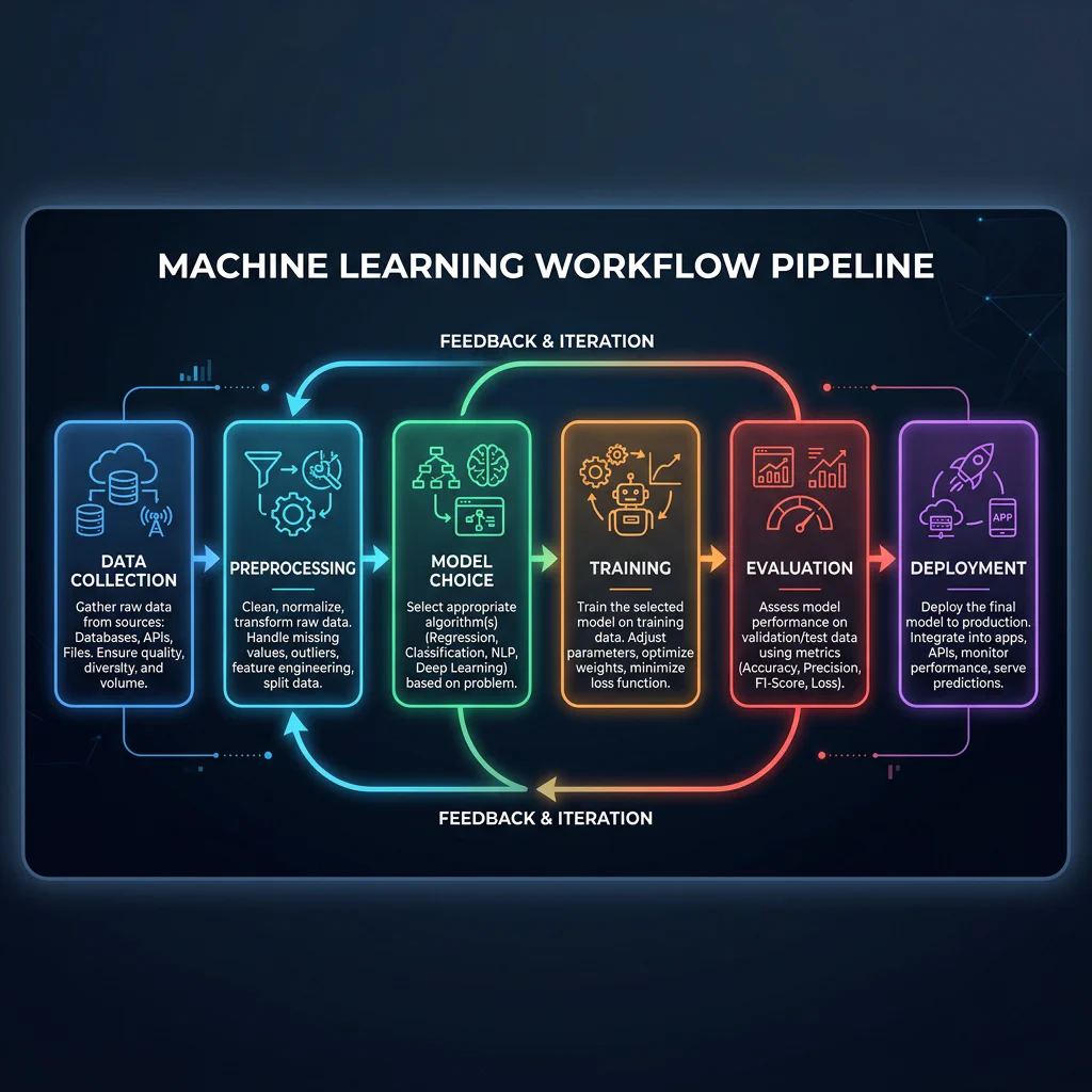
Machine Learning Workflow Pipeline
Slide 30: Model Deployment: Model Packaging & Export
- Slide Title: Model Deployment: Model Packaging & Export
- Core Concepts:
- Model Serialization: Converting a trained in-memory Python object into a persistent file artifact.
- Serialization Libraries: Using
jobliborpicklefor scikit-learn classifiers, or compiling toONNXfor multi-platform neural networks. - Walkthrough Steps:
- Train and validate the machine learning model.
- Save the trained model parameters to disk (e.g.,
model.joblib).
Slide 31: Model Deployment: Inference API Deployment
- Slide Title: Model Deployment: Inference API Deployment
- Core Concepts:
- API Definition: Exposing the model’s prediction functions behind a REST API for consumption by external applications.
- Framework Choice: Using Python web frameworks like Flask or FastAPI.
- Walkthrough Steps:
- Load the serialized model artifact inside a Flask web application on startup.
- Expose prediction functionality through a
/predictREST API endpoint. - Receive input features, perform inference, and return predictions as real-time JSON responses.
09. Recap, Quiz & Live Q&A (00:58 – 01:00)
Slide 32: Mapping Tasks & Tools to the Pipeline
- Slide Title: Mapping Tasks & Tooling
- Ecosystem Stack: Pandas, NumPy, Scikit-Learn, TensorFlow, PyTorch, MLflow.
Slide 33: Wrap-Up Key Takeaways
- Slide Title: Wrap-Up Key Takeaways
- Key Summary: Define problem paradigm first, start with simple baselines, data preprocessing determines 90% of model performance.
Slide 34: Visual Cheat Sheet Summary
Slide Title: Visual Cheat Sheet Summary
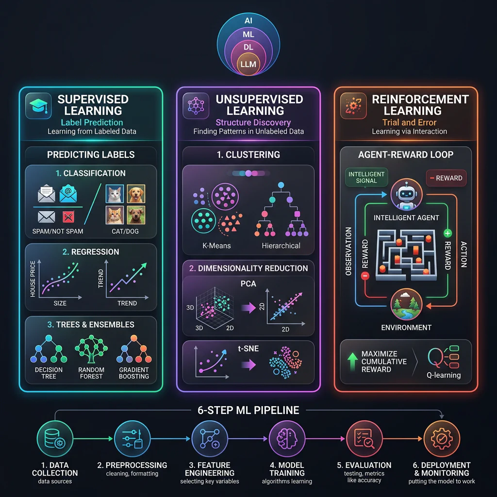
Session Infographic
Slide 35: Summary Quiz: Paradigm Matchmaker
- Slide Title: Summary Quiz: Paradigm Matchmaker
- Scenarios Covered:
- Car steering learning via cones feedback (Reinforcement).
- Predict job posting salary (Supervised).
- Find transaction fraud groups without labels (Unsupervised).
Slide 36: Audience Live Q&A
Slide Title: Audience Q&A
Key Prompts: Handling imbalanced classification datasets, deep learning fits, career transition paths.

Audience Q&A Background illustration