Introduction to Machine Learning & Modelling Techniques
Supervised, Unsupervised & Reinforcement Learning
A 1-hour conceptual masterclass designed for beginner-to-intermediate data professionals to build an intuitive, visual, and practical mental map of ML algorithms.

Navigating the AI Ecosystem
- Artificial Intelligence (AI): The overarching field of creating systems that mimic human intellect (includes search, heuristics, planning).
- Machine Learning (ML): Systems learning rules and functions directly from structured datasets without manual programming.
- Deep Learning (DL): Nested layers of neural networks learning complex patterns from raw unstructured data.
- Large Language Models (LLM): Transformer-based generative AI systems understanding human text sequences.

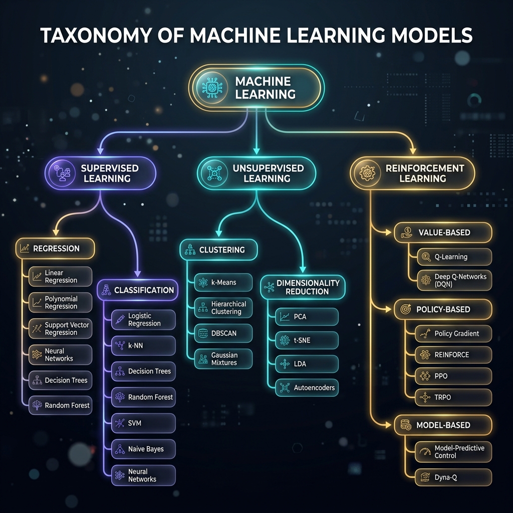
The Three Pillars of ML
- Supervised Learning: Training model parameters using paired input-output datasets to
predict numeric labels or classes.
Example: Predicting customer default risk using historical loan details.
- Unsupervised Learning: Organizing unlabeled data into natural partitions, dimensions,
or clusters without human correction.
Example: Grouping buyers into behavioral segments based on shopping habits.
- Reinforcement Learning: An active agent optimizing behavioral policies inside
environments using trial-and-error rewards.
Example: Training a robot vacuum to navigate a room using pathfinding rewards.
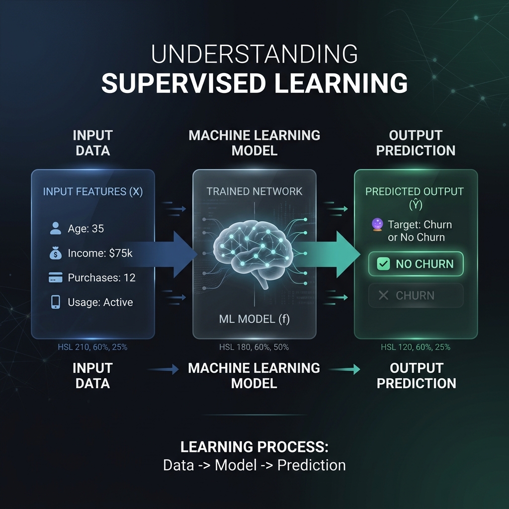
Supervised Learning Basics
- Core Goal: Learn an approximation function Y = f(X) where X are inputs and Y are target labels.
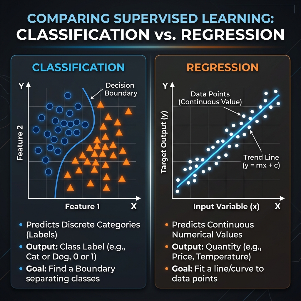
- Regression: The target label is a continuous numeric value.
Examples: Estimating real estate market prices or tracking server CPU temperatures.
- Classification: The target label is a discrete categorical bucket.
Examples: Flagging transaction fraud or sorting incoming emails into spam folders.
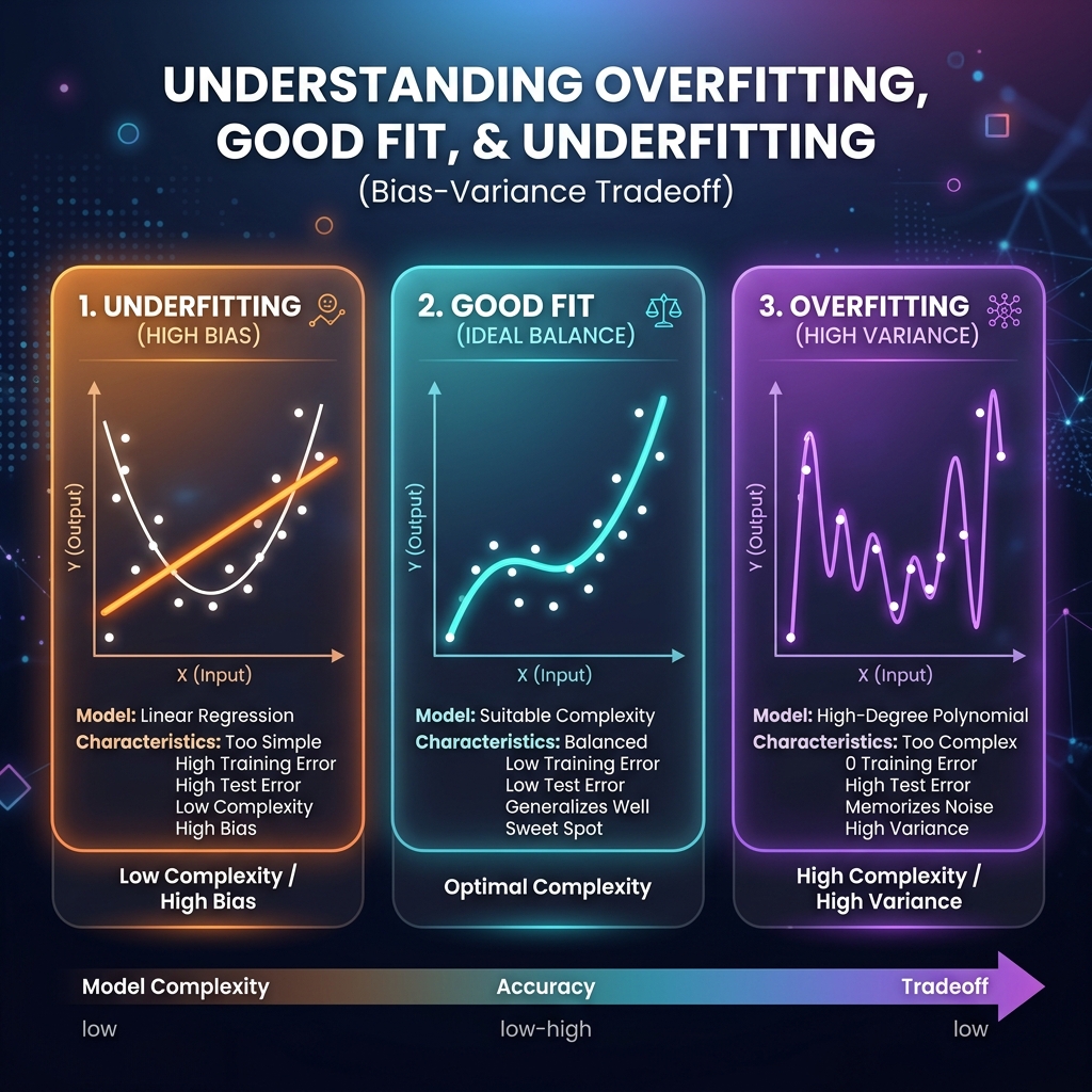
Bias, Variance & Model Tuning
- Underfitting (High Bias): The model is too simple to capture underlying patterns.
Example: Predicting house price using only size, ignoring location. The model is too rigid.
- Overfitting (High Variance): Model memorizes training noise and outliers.
Example: Fitting a high-degree polynomial that matches every single outlier, but fails on new houses.
- Cross-Validation: Splitting data into k-folds to validate model performance.
Example: Splitting data into 5 groups, training on 4, testing on 1, and rotating 5 times to prevent bias.
- Hyperparameter Tuning: Adjusting model options before training to control complexity.
Example: Limiting a decision tree's depth to 3 levels, or setting k = 5 in k-NN to smooth out predictions.
Ordinary Least Squares (OLS)
The math behind standard Linear Regression. We fit a linear function and optimize parameters by minimizing the Mean Squared Error (MSE) loss function:
Cost Function: MSE = (1/n) * Σ (yᵢ - ŷᵢ)²
- yᵢ is the true target, ŷᵢ is the model prediction.
- Minimizing MSE yields the line of best fit (least squares residuals).

🏠 Intuitive Real-World Example
Predict Housing Price (y, Dependent Variable) based on House Size (x₁, Independent Variable). The weight β₁ represents the price increase per additional sq. ft. (e.g., +$250/sq.ft.), while β₀ (intercept) is the base land cost.
Regularization Math
To prevent overfitting, we add a coefficient magnitude penalty term (α) to the OLS cost function:
Ridge (L2 Penalty) Cost:
Lasso (L1 Penalty) Cost:

📉 Regularization & Weight Shrinkage
If predicting housing price using Size, Bedrooms, and Wall Color: a high penalty α shrinks weights. Ridge (L2) shrinks weights evenly (retaining all features), while Lasso (L1) drives Wall Color's weight to exactly zero, automatedly discarding it.
Classification: Part 1
- Logistic Regression: Fits features through a sigmoid activation curve to predict
category probabilities between 0 and 1.
Example: Predicting if a client defaults on a loan (Probability 0 to 1).
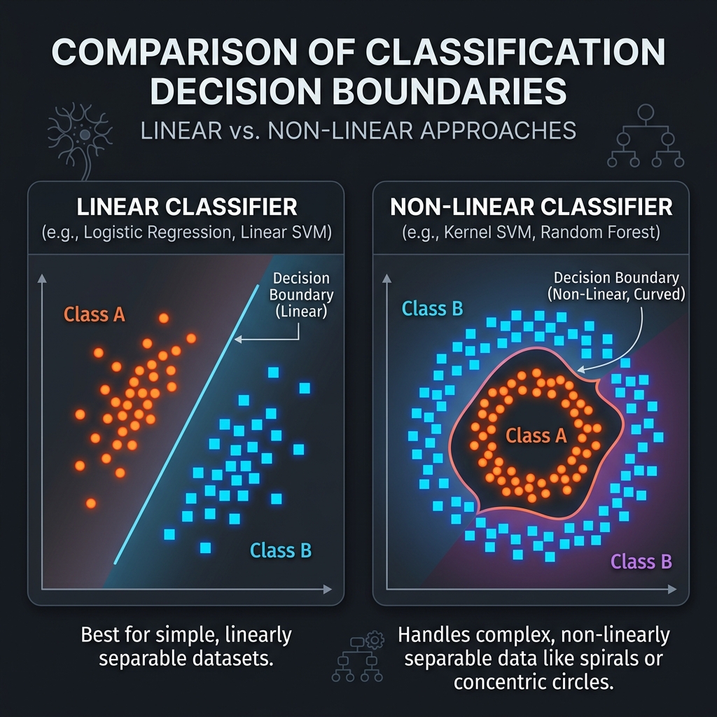
- Support Vector Machines (SVM): Solves optimal linear boundaries by maximizing margins
separating data coordinate groups.
Example: Classifying handwritten letters by drawing widest boundary corridors.
Distance-Based: k-NN
- k-Nearest Neighbors (k-NN): Classifies points based on the majority labels of the 'k' closest points in coordinates space.
- Details: Requires no mathematical training beforehand (lazy learner), but is computationally expensive for large tables.
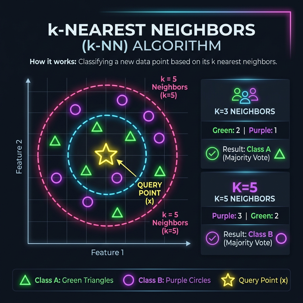
🏨 Intuitive Hotel Classification Example
To classify a new hotel based on Price per Night ($) and Distance to Beach (meters) under k=5: locate the 5 nearest hotels in coordinate space. If 4 are "Budget Hostel" and 1 is "Luxury Resort", the model classifies the new hotel as Budget Hostel by majority vote.
k-NN: Step-by-Step Example
Classifying a new fruit (Sweetness = 6, Crunchiness = 4) with k = 3 neighbors.
1. Measure Distance (Euclidean)
Formula: Distance = √((x₂ - x₁)² + (y₂ - y₁)²)
| Fruit | Sweet (x) | Crunch (y) | Calculation | Distance |
|---|---|---|---|---|
| Apple A | 7 | 7 | √((7-6)² + (7-4)²) = √(1+9) | 3.16 |
| Apple B | 8 | 5 | √((8-6)² + (5-4)²) = √(4+1) | 2.24 |
| Orange A | 3 | 3 | √((3-6)² + (3-4)²) = √(9+1) | 3.16 |
| Orange B | 7 | 2 | √((7-6)² + (2-4)²) = √(1+4) | 2.24 |
| Orange C | 6 | 2 | √((6-6)² + (2-4)²) = √(0+4) | 2.00 |
2. Find 3 Neighbors
- Orange C (Dist: 2.00)
- Apple B (Dist: 2.24)
- Orange B (Dist: 2.24)
3. Vote for Class
- Oranges: 2 votes (C, B)
- Apples: 1 vote (B)
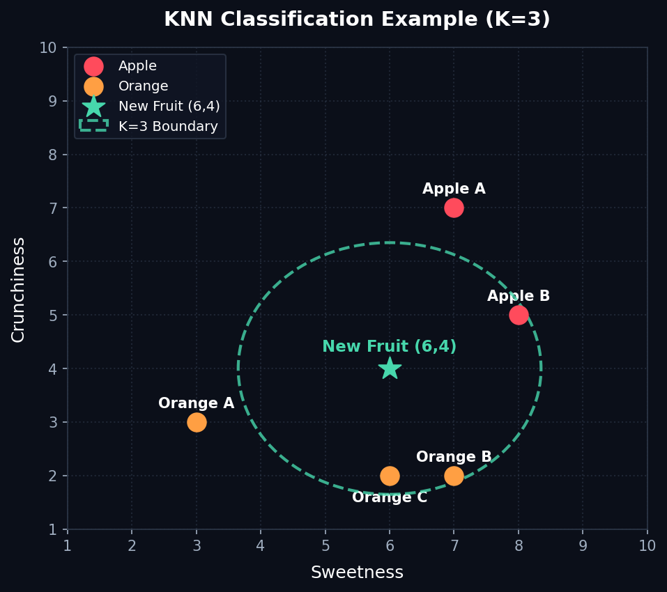
✅ Final Classification
The new fruit is classified as an Orange because it secured the majority of the votes (2 out of 3).
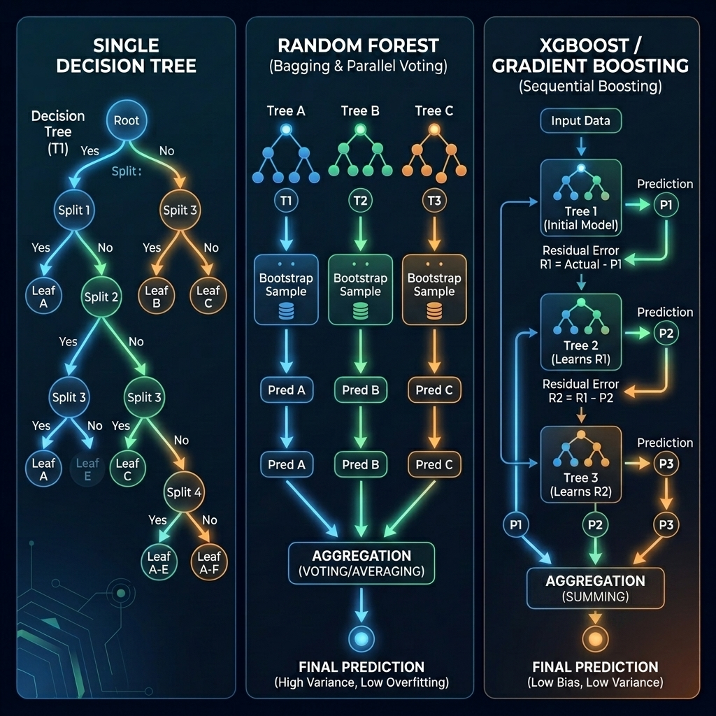
Tree-Based Ensembles
- Decision Trees: A hierarchical sequence of logic cuts (rules) dividing features into homogeneous groups.
- Random Forest (Bagging): Aggregates many trees trained on random sample subsets, voting in parallel to reduce variance.
- XGBoost (Extreme Gradient Boosting): Sequentially fits trees where each new model corrects residuals (mistakes) of the previous tree.
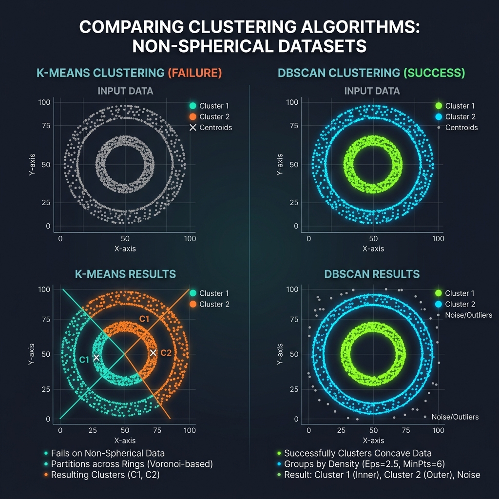
Clustering Algorithms
- K-Means: Groups data points into k spherical partitions by iteratively relocating centroids to match local means.
- Hierarchical Clustering: Builds nested tree branches (agglomerative) to connect data coordinates without predefining cluster counts.
- DBSCAN (Density-Based Spatial Clustering of Applications with Noise): Groups dense coordinate neighborhoods, discovering arbitrary cluster shapes and isolating sparse noise.

K-Means: Step-by-Step Example
Grouping customers into K = 2 clusters based on Age and Spending Score (1-10). Initial centroids: C1 = (20,3), C2 = (40,8).
1. Distance Assignment Step
| Customer | Age (x) | Spend (y) | Dist to C1 (20,3) | Dist to C2 (40,8) | Cluster |
|---|---|---|---|---|---|
| User A | 22 | 4 | 2.24 | 18.44 | C1 |
| User B | 28 | 2 | 8.06 | 13.42 | C1 |
| User C | 45 | 9 | 25.71 | 5.10 | C2 |
| User D | 38 | 7 | 18.44 | 2.24 | C2 |
2. Update Centroid Center Step
- New C1 Center: Average of User A(22,4) & B(28,2) → ((22+28)/2, (4+2)/2) = (25, 3)
- New C2 Center: Average of User C(45,9) & D(38,7) → ((45+38)/2, (9+7)/2) = (41.5, 8)

🔄 3. Repeat Until Convergence
Steps 1 & 2 are repeated with updated centroids. The process stops when cluster assignments freeze and centroids no longer shift coordinate positions.
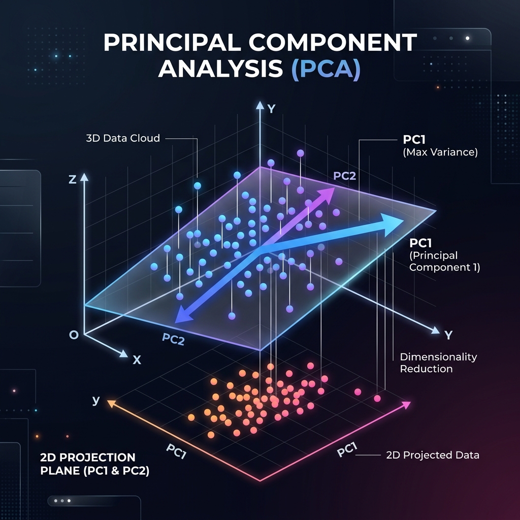
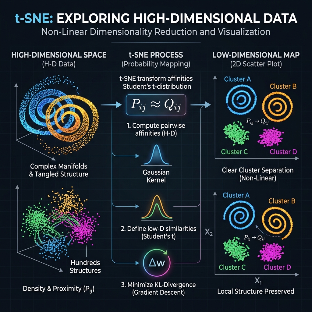
Dimensionality Reduction
- PCA (Principal Component Analysis): Projects high-dimensional data orthogonally to new directions capturing maximum variance.
- t-SNE (t-Distributed Stochastic Neighbor Embedding) / UMAP (Uniform Manifold Approximation and Projection): Non-linear manifold mapping that preserves local neighborhoods to visualize distributions in 2D coordinate space.
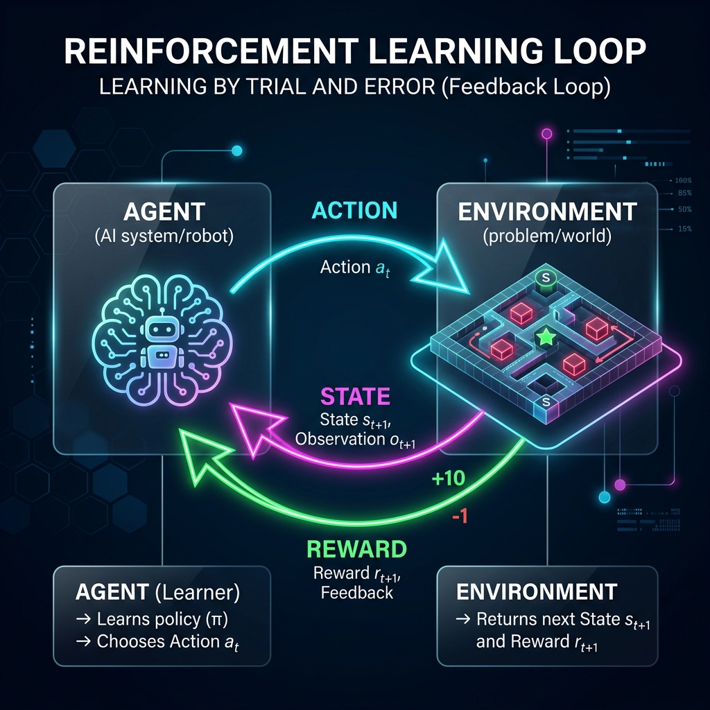
Reinforcement Learning Basics
- Concept: Teaching model behaviors using feedback loops based on action trials and environmental rewards.
- Agent: The core decision-making AI engine.
- Environment: The interactive space surrounding the agent.
- State: Current environmental configurations.
- Action: Movement selection performed by the agent.
- Reward: positive or negative numeric feedback score.
Interactive: RL Agent Learning Journey
Exploration Blind Trial: The robot moves forward, enters a hazard zone (fire), and immediately receives a large negative reward (-100). The agent updates its memory weights to avoid this action in similar grid states in future epochs.

Exploitation Path Corrected: After multiple iterations, the agent learns the barrier locations, navigates around hazard areas, reaches the battery charger goal, and earns a positive reward (+100).

How Many Models Exist?
There is no fixed count, but models group into 5 core families:
- 📉 Linear Models: Fit flat linear planes (e.g. Linear/Logistic, Ridge/Lasso, and Polynomial Regression).
- 🌲 Tree-based Ensembles: Cut spaces into nested step rules (e.g. Decision Trees, Random Forests, XGBoost).
- 📏 Distance & Kernel Models: Proximity distance & coordinate projections (e.g. k-NN, Kernel SVM, K-Means, DBSCAN).
- 🎲 Probabilistic Models: Rely on bayesian probability weights (e.g. Naive Bayes, GMM).
- 🕸️ Neural Networks: Deep nodes layers mapping non-linear inputs to outputs.
* Key Contrast: While Linear Models assume flat, straight-line relationships (with Polynomial mapping non-linear relations using linear solvers), Tree Ensembles, Kernels, and Neural Networks are inherently Non-Linear—allowing them to fit complex curved boundaries.
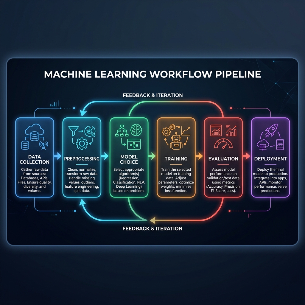
The 6-Step ML Workflow
- Data Collection: Querying raw database storage tables or APIs.
- Preprocessing: Cleaning outliers, scaling values, feature engineering.
- Model Choice: Picking the target mapping algorithm class.
- Training: Fitting candidate model weights on data splits.
- Evaluation: Validating output accuracy metrics on test folds.
- Deployment: Packaging final models into live inference APIs.
Visual Cheat Sheet Summary

Audience Q&A
Ask Me Anything!
Suggested Topics to Start:
- How to manage imbalanced label coordinates?
- When is deep neural computing actually necessary?
- Transition paths from traditional BI analytics to ML engineering.
